Coupling package

The work share between both modules is as follows:

• The connections module shall deal with the topological details of the junction, for example length, angle, orientation connected systems.

• The junctions module deals with the physics of wave transmission over the coupling.

Connections

Due to the fact that the current examples are rather simple and that there is no geometry description of systems available this module is just there to establish the logical structure of future developments.

This will be for example the connection geometry of plate connections that provide the length of the connection and the angle of each connected plate. These geometrical parameters serve as input for the junction classes.

Junctions

Junctions deal with the transmission or exchange of wave field power. The complex and detailed physics is described in many references and presented in chapter 8 of [Pei2022].

One special feature of pyva is that the coupling loss factors are calculated bases on the diffuse field reciprocity theorem from Shorter [Sho2005] and the hybrid FEM/SEA theory that is also an excellent and straightforward approach for the calculation of coupling loss factors (CLF).

In the result this does not change too mach, except for line junctions. Here, the reverberant field cannot be separated in longitudinal, shear and bending waves. For very specific reasons that are explained in [Pei2022] the system plate contains in-plane (longitudinal plus shear) and bending-waves. In classical wave transmission SEA [Lan1990] this is not required.

In general all junctions are defined by their connected systems. Thus, there is an abstract base class pyva.coupling.Junction that contains all methods and parameters that are common for all subclasses.

To each junction a specific set of degrees of freedom is defined in accordance with the definition for One dimensional acoustic systems. The ID, wave_DOF and DOFtype are determined in the order of the connected systems. Not that wave_DOF have a slightly different meaning that deterministic DOFs.

pyva.coupling.junctions.Junction.get_wave_DOF() is used to provide exactly this degrees of freedom and that are store in the attribute wave_DOF of each junction. Based on this method there are the pyva.coupling.junctions.Junction.res_DOF() and meth:pyva.coupling.junctions.Junction.exc_DOF methods that provide the degrees of freedom that are used for the creation of the junction_matrix. The junction_matrix is it the matrix that is the part of equation (3) that is added to the full SEA model setup. Thus, the junctions are playing the role of elements in the SEA system context beause they determine the energy flow between the systems.

The properties N and N_wave provide the number of physical connected systems or wave fields, respectively.

Line Junction

Line junctions couple two dimensional subsystems. Most information comes from the connected systems itself. They define by their degrees of freedom which wave fields are coupled. Unfortunately, there is no simple and analytical point force response function, so discrete radiation stiffness matrices cannot by calculated easily. Hence, the line junction algorithm is based on wavenumber coordinates in the line direction and the CLF is calculated from diffuse field angular averaging.

Even though the parameters of the junction: length and the angles of connected subsystems the theory behind this type of junction is very complex. Thus, there are several versions for the calculation of the transmission coefficients.

The main and important methods are transmission_wavenumber() and transmission_wavenumber_diffuse() that use the CLF implementation as shown in [Pei2022]. However, there are additional methods for validation purpose: The transmission_wavenumber_langley() using Langleys implementation [Lan1990] and transmission_wavenumber_wave() that shows my struggle with a simple application by simply using the hybrid coupling loss factor implementation, that is not possible as shown in detail in [Pei2022].

Sketch of line junction set-up.

For junction example we require the following imports

import pyva.coupling.junctions as jun
import pyva.properties.structuralPropertyClasses as stPC
import pyva.systems.structure2Dsystems as st2Dsys
import pyva.data.matrixClasses as mC
import pyva.properties.materialClasses as matC

import pyva.useful as uf

using the typical SEA third octave frequencies

# x-axis tics
fc,fclabels = uf.get_3rd_oct_axis_labels()

For the creation of a junction some systems must be created

# Plate dimensions
Lx1 = 2.5
Lx2 = 1.7
Ly = 1.7
area1 = Lx1*Ly
area2 = Lx2*Ly

# Create materials
alu = matC.IsoMat(nu=0.3,eta = 0.0)

# Create props
alu1mm = stPC.PlateProp(0.001,alu)
alu2mm = stPC.PlateProp(0.002,alu)

# Create plate subsystems
plate1 = st2Dsys.Structure2DSystem(1,area1,alu1mm)
plate2 = st2Dsys.Structure2DSystem(2,area2,alu2mm)

As discussed the junction requires angles

# junction properties
angle1 = 0
angle2 = 90*np.pi/180

and length and is created by using the LineJunction constructor

J12 = jun.LineJunction((plate1,plate2),Ly,(angle1,angle2))
>>> J12
LineJunction with systems:
SEA_system with ID:1        reverberant wave_DOF(s):[3 5] angle: 0.0000
SEA_system with ID:2        reverberant wave_DOF(s):[3 5] angle: 1.5708
length       : 1.7

The physical wave_DOFs are determined by

>>> dofs = J12.wave_DOF()
>>> dofs
DOF object with ID [1 1 2 2], DOF [3 5 3 5] of type [DOFtype(typestr='velocity'), DOFtype(typestr='velocity'), DOFtype(typestr='velocity'), DOFtype(typestr='velocity')]

The DOFs of the junction- or SEA-matrix of the junction are given by

>>> J12.res_DOF
DOF object with ID [1 1 2 2], DOF [3 5 3 5] of type [DOFtype(typestr='energy')]
>>> J12.exc_DOF
DOF object with ID [1 1 2 2], DOF [3 5 3 5] of type [DOFtype(typestr='power')]

Those are used in the junction_matrix that is gerated by

>>> JM = J12.junction_matrix(np.array([1000,2000]))
LinearMatrix of size (4, 4, 2), sym: 1
DataAxis of 2 samples and type general
resdof: DOF object with ID [1 1 2 2], DOF [3 5 3 5] of type [DOFtype(typestr='energy')]
excdof: DOF object with ID [1 1 2 2], DOF [3 5 3 5] of type [DOFtype(typestr='power')]

Due to the degrees of freedom handling of the DynamicMatric class the junction matrix can simply be added to the SEA matrix. An impression of the complicated wave transmission can by achieved by showing the angular dependency of the transmission. We determine the maximum wavenumber by the slowest wave type; the bending on the thin plate

omega0 = 5000*2*np.pi
max_k = alu1mm.wavenumber_B(omega0)

kx = np.linspace(0.,max_k,200)

The method provides the output as signal if not requested differently by signal = False so with

tau5000 = J12.transmission_wavenumber(omega0,kx,(0,1), i_in_wave = (3,3,5,5) , i_out_wave= (5,3,5,3))
tau5000.plot(1)

we get the various shapes of the transmission coefficients

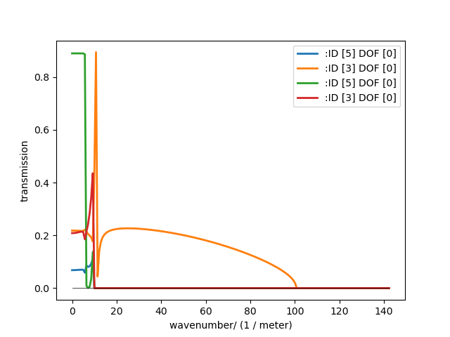
Angular wave transmission of line junction.

The diffuse transmission coefficient, that provides the CLF at the end is determined by

omega = mC.DataAxis.octave_band()
taus = J12.transmission_wavenumber_diffuse(omega.angular_frequency, (0,1), i_in_wave = (3,3) , i_out_wave= (5,3))

Leading to following transmission coefficients

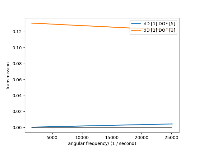
Diffuse wave transmission of line junction.

Area Junction

Area junction deal with the acoustic power flow between plates and/or cavities. This can be (c) a direct connection of connected cavities (which tends to violate the low coupling assumption of SEA), (a,b) a plate connected to a cavity or (d) two cavities that are connected via a plate.

In Possible system combinations for area junctions. the available options are shown.

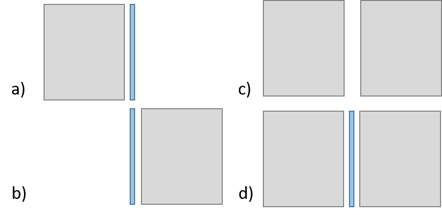
Possible system combinations for area junctions.

The area junction is special is such a way that the physics of noise transmission require the violation of the base rule of SEA that only neighbour subsystems can exchange energy. The noise transmission via walls or plates includes the forced motion of the plate, better known as the mass law. Thus an area junction in a cavity-plate-cavity configuration has an extra and direct transfer path; the non-resonant path that takes care of the mass law.

Sketch of area junction set-up.

As shown in the Example: Two rooms separated by a wall area junction is created by a list or tuple of the three subsystems. Please not that the plate system must be the centre system when three are involved

J123 = con.AreaJunction((room1,wall,room2))

If not mentioned differently the area is taken from the plate. For pure cavity connections the area must be given. Because of the fact that there are multiple transfer paths the transmission coefficient must be calculated by creating a test setup as shown in the example.

When the plate is covered with noise control treatment this is automatically considered fron the definition of the SEA plate system. The cavity-plate side corresponds to the index 0 in the trim tuple of the plate. The plate-cavity side to the index 1.

Hybrid area junction

The hybrid area junction is created in such a way that a flat FE-model radiates into the connected cavities.

Sketch of Hybrid area junction set-up.

The contructor requires the connected SEA systems, the trim if applicable and the FE-model that represents the centered plate. Due to the current simplistic implementation of FE-models the mesh is always supposed as regular mesh.

The use of the constructor is given in example Two rooms with FE-plate.

HJ123 = jun.HybridAreaJunction((room1,room2),plateFE)

In contrast to SEA area junctines the trim must be explicitely defined with:

HJ123_trim = con.AreaJunction((room1,wall,room2),trim={None,my_NCT})

The major method is pyva.coupling.junctions.HybridAreaJunction.CLF(). In contrast to the pure SEA method there are additional outputs:

eta, eta_alpha = HJ123.CLF(omega.angular_frequency)

The eta_alpha return value provides the additional damping of the connected SEA systems due the damping in the FEM-system.

For practical reasons a force is implemented junction method so that force loads of the FE-model are considered in the full hybrid solution. In this case further additional output arguments are required:

eta, eta_alpha, power_in, modal_disp = HJ123.CLF(omega.angular_frequency, force = 1N@Node200)

Due to the fact that the reverberant fields in the cavities excite the FEM-system one further method is neccessary. This is FEM_response() that calculates the modal cross spectral density of FEN-system due to the energy in the connected SEA systems:

Sqq = FEM_response(omega,energy)

Semi infinite fluid

The semi infinite fluid is in principle a acoustic half space, thus a way to model the radiation of SEA systems into the free space. It is a subclass of the area junction, because it is like an area junction with the free space as third cavity. So there is no power transfer back and the radiation is considered as an additional (radiation) damping loss in the SEA matrix.

A typcial SIF definition looks like a junction creation where the (last) cavity subsystem is replaced by a fluid:

# create semi infinite fluids
sif1 = jun.SemiInfiniteFluid((room,plate1), air)

How SIFs are used can be seen in Box cover of sound source.