Data package

The data modules of pyva have one main purpose: They shall represent the following linear system of equations that represent the discrete form of the equations of motion.

One typical example is given in equation (1).

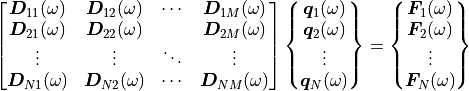
(1) $\begin{bmatrix} \boldsymbol{D}_{11}(\omega) & \boldsymbol{D}_{12}(\omega) & \cdots & \boldsymbol{D}_{1M}(\omega) \\ \boldsymbol{D}_{21}(\omega) & \boldsymbol{D}_{22}(\omega) & & \boldsymbol{D}_{2M}(\omega) \\ \vdots & \vdots & \ddots & \vdots \\ \boldsymbol{D}_{N1}(\omega) & \boldsymbol{D}_{N2}(\omega) & \cdots & \boldsymbol{D}_{NM}(\omega) \\ \end{bmatrix} \begin{Bmatrix} \boldsymbol{q}_1(\omega) \\ \boldsymbol{q}_2(\omega) \\ \vdots \\ \boldsymbol{q}_N(\omega) \end{Bmatrix} = \begin{Bmatrix} \boldsymbol{F}_1(\omega) \\ \boldsymbol{F}_2(\omega) \\ \vdots \\ \boldsymbol{F}_N(\omega) \end{Bmatrix}$

$\boldsymbol{D}_{ij}(\omega)$ are the coefficients of the dynamic stiffness matrix, $\boldsymbol{q}_{i}(\omega)$ the qeneralised displacement degrees of freedom and $\boldsymbol{F}_{i}(\omega)$ the generalized forces.

The first idea might be to use numpy arrays for both the matrices and the vectors but the properties of both motivate the introduction of new classes to handle them more efficiently. The dynamic stiffness matrix is frequency dependent and therefore a three-dimensional array, the generalized vector becomes two-dimensional. In addition typical matrices have symmetry properties. Thus, the full storage of symmetric, hermitian, diagonal or sparse matrices would be inefficient. Furthermore, every degree of freedom belongs to a certain node with location in space and local degrees of freedom such as displacements in x-, y- or z-directions. These degrees of freedom must be efficiently managed, meaning that the index and positioning of each degree of freedom in the matrices and vectors must be dealt with.

For the matrices this motivated the introduction of the LinearMatrix and the DynamicMatrix class. The first class aims at the consideration of symmetry and frequency dependence and the latter at relating each index in the matrix to a specific degreed of freedom. By using the above matrix classes the user shall not care too much about the symmetry because the implementation will automatically care about this and find the best solution for storing the data. The generalized vector is represented by the Signal class.

Vibroacoustic models are usually based on meshes, thus the physical domain is discretized into several elements whose vertices are represented by nodes. Every node has many local degrees of freedom (for example the displacement in x- and y- direction) and a physical quantity (for example pressure, displacement or force). The class that organises this topic is the DOF class. The type attribute of the DOF class consists of a further class called DOFtype. This class deals with unit and the physical type of degrees of freedom. For example the physical quantity length hat unit meter.

DOFtype

The most basic level of data handling is performed by the DOFtype class. This class uses many internal attributes in order to handle units and physical quantities and operations with them.

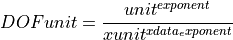
This class is organised as a fraction to allow for the treatment of spectral density. The following formula shows the meaning of the object attributes:

(2) $DOFunit = \frac{unit^{exponent}}{xunit^{xdata_exponent}}$

The unit is given by the type or typestring, e.g.

The related module is imported by:

>>> import pyva.data.dof as dof

Let’s start with an example to clarify the content. A force is defined by the acceleration it performs on a mass. So the physical quantity force hat the unit Newton that can also by expressed as units of kg*meter*sec^-2 of the base quantities: length, mass and time.

The easiest way to create an instance of the physical quantity force by using the DOFtype constructor with typestr keyword:

>>> force = dof.DOFtype(typestr='force')

creating the following output:

>>> force
force in newton

Now let’s check the exponents of the base quantities using the method LMT:

>>> force.LMT
array([ 1,  1, -2])

Meaning

${\rm Newton} = \frac{\rm kg \quad m}{\rm s^2}$

Imagine that we create an area:

area = dof.DOFtype(typestr='area')

It is well known that pressure is defined as force per area:

>>> pressure = force/area
>>> pressure
force/area**1 in newton/meter ** 2

This can alternatively be created directly by:

>>> pressure_ = dof.DOFtype(typestr = 'pressure')

Now, the DOFtype class knows the pressure origin and uses the unit for pressure:

>>> pressure_
pressure in pascal

However, division gives a no unit quantity:

>>> pressure_/pressure
unknown

On the other hand, multiplying a pressure by the area provides the force:

>>> pressure*area
force in newton

Many other methods are useful for label generation, so the label of the pressure would give:

>>> pressure_.label()
'pressure/ (pascal)'

Degree of freedom DOF

The DOF class adds the node ID and the local degreed of freedom to the DOFtype. Thus, the DOF class provides an ID, an orientation and a physical unit for every degree of freedom. Note that the DOF class is without a mesh functionality. Thus, it purely manges the ID of the degrees of freedom. In figure Sketch of nodal degree of freedom. the DOF attributes are sketched.

_images/dof.png — Sketch of nodal degree of freedom.

ID defines the node by a positive integer > 0
dof the local DOF or orientation,
- 0: scalar, no orientation, e.g. pressure, temperature
- 1-3: for the three space axis.
- 4-6: for rotations around the three space axis
type: DOFtype of node

Internally the ID and the dof are ndarrays of int. The type attribute is a list of DOFtype object. Normally all attributes must have the same size, except when the constructor is used with repetition=True option.

Before creating a DOF instance, a DOFtype instance is required:

>>> import pyva.data.dof as dof
>>> force = dof.DOFtype(typestr='force')
>>> dof.DOFtype(typestr='displacement')

Next, we create appropriate ID and ldof arrays:

>>> ID   = np.arange(1,3)
>>> ldof = np.arange(1,4)

>>> ID   = np.repeat(ID,3)
>>> ldof = np.tile(ldof,2)

>>> ID
array([1, 1, 1, 2, 2, 2])
>>> ldof
array([1, 2, 3, 1, 2, 3])

A pure displacement DOF vector is created by:

>>> my_dof = dof.DOF(ID,ldof,disp)
>>> my_dof
DOF object with ID [1 1 1 2 2 2], DOF [1 2 3 1 2 3] of type [displacement in meter]

The same can be created using the repetition argument:

>>> my_dof = dof.DOF([1,2],[1,2,3],disp, repetition = True)
>>> my_dof
DOF object with ID [1 1 1 2 2 2], DOF [1 2 3 1 2 3] of type [displacement in meter]

Every combination of IDs, dofs and DOFtypes is possible:

>>> many_dof = dof.DOF([1,1,2,2],[1,2,3,1],[disp,disp,force,force])
>>> many_dof
DOF object with ID [1 1 2 2], DOF [1 2 3 1] of type [displacement in meter, displacement in meter, force in newton, force in newton]

Useful and important functions are the indexing, for example when the index of subsets is required

>>> my_part_dof = dof.DOF([1,2],[2],disp,repetition = True)
>>> ix = my_dof.index(my_part_dof)
>>> ix
array([1, 4], dtype=int64)

This index can be used to extract the dofs from the main set:

>>> my_dof[ix]
DOF object with ID [1 2], DOF [2 2] of type [displacement in meter]

This is useful when indexes into system matrices are required.

DataAxis

In contrast to degrees of freedom classes the DataAxis class provides information about the third dimension of the vibroacoustic system. In most cases this is frequency, but it can also be time, wavenumber or other quantities.

The DataAxis has the attributes data and the type. The constructor works with all typical input of DOFtype arguments.

A frequency axis is generated by:

>>> freq_axis  = mC.DataAxis(np.arange(0.,2.,0.1),typestr = 'frequency')
>>> freq_axis
DataAxis of 20 samples and type frequency in hertz

A useful method is the angular_frequency() method that always provides the data in angular units:

>>> freq_axis.data
array([0. , 0.1, 0.2, 0.3, 0.4, 0.5, 0.6, 0.7, 0.8, 0.9, 1. , 1.1, 1.2,
   1.3, 1.4, 1.5, 1.6, 1.7, 1.8, 1.9])
>>> freq_axis.angular_frequency
array([ 0.        ,  0.62831853,  1.25663706,  1.88495559,  2.51327412,
        3.14159265,  3.76991118,  4.39822972,  5.02654825,  5.65486678,
        6.28318531,  6.91150384,  7.53982237,  8.1681409 ,  8.79645943,
        9.42477796, 10.05309649, 10.68141502, 11.30973355, 11.93805208])

Signal

The Signal sequence of a physical quantity of managed by the Signal class. The rows of the two-dimensional array represent the sequence over the DataAxis for every degree of freedom.

The signals are given as ydata in a two dimensional aray, the xdata attribute determines the xaxis and the dof links every row to one specific degree of freedom:

>>> p_dof = dof.DOF([1,2],[0,0],dof.DOFtype(typestr = 'pressure'))
ydata = np.array([np.sin(omega),np.cos(omega)])

A Signal is then constructed by:

>>> sig1 = mC.Signal(freq_axis,ydata,p_dof)
>>> sig1
Signal object of 20 samples with 2 channels and properties ...
DataAxis of 20 samples and type frequency in hertz
DOF object with ID [1 2], DOF [0 0] of type [pressure in pascal]

A quite useful method is the plot method:

>>> sig1.plot(1)

Leading to:

Until now we have explained the required classes to handle the vector types of the dynamic equation (1).

LinearMatrix

The LinearMatrix class aims at efficient handling of complex matrices that change over frequency or sometimes other parameters like time or wavenumber. In order to present the functionality we create some test data:

>>> from pyva.data import matrixClasses as mC
>>> import numpy as np

>>> data = np.arange(18).reshape(3,3,2)
>>> data[:,:,0]
array([[ 0,  2,  4],
       [ 6,  8, 10],
       [12, 14, 16]])

A linear matrix can be generated by calling the constructor with this input:

>>> lin_data = mC.LinearMatrix(data)
>>> lin_data
LinearMatrix of size (3, 3, 2), sym: 0
First matrix up to index 5 at iz = 0
[[ 0  2  4]
 [ 6  8 10]
 [12 14 16]]

Shape and symmetry are denoted in the output. When we create a symmetric matrix with:

>>> sym_data = (data + data.transpose(1,0,2))/2
>>> sym_data[:,:,0]
array([[ 0.,  4.,  8.],
       [ 4.,  8., 12.],
       [ 8., 12., 16.]])
>>> lin_sym_data = mC.LinearMatrix(sym_data)
>>> lin_sym_data
LinearMatrix of size (3, 3, 2), sym: 1
First matrix up to index 5 at iz = 0
[[ 0.+0.j  4.+0.j  8.+0.j]
 [ 4.+0.j  8.+0.j 12.+0.j]
 [ 8.+0.j 12.+0.j 16.+0.j]]

The constructor identifies the symmetry automatically. The same happens for hermitian and diagonal data:

>>> one = np.eye(3)
>>> mC.LinearMatrix(one)
LinearMatrix of size (3, 3, 1), sym: 3
First matrix up to index 5 at iz = 0
[[1.+0.j 0.+0.j 0.+0.j]
 [0.+0.j 1.+0.j 0.+0.j]
 [0.+0.j 0.+0.j 1.+0.j]]

For efficiency reasons, only the upper triangle of symmetric and hermitian matrices can be given:

>>> triu_data = np.arange(6).reshape(6,1)
>>> mC.LinearMatrix(triu_data, sym = 1, shape = (3,3,1))
LinearMatrix of size (3, 3, 1), sym: 1
First matrix up to index 5 at iz = 0
[[0.+0.j 1.+0.j 2.+0.j]
 [1.+0.j 3.+0.j 4.+0.j]
 [2.+0.j 4.+0.j 5.+0.j]]

See the numbering of the upper coefficients to understand the indexing. Here 6/9-th of coefficients is required to store the data. Slicing and indexing works similar to ndarrays.

>>> lin_sym_data[0:2,0:2,1]
LinearMatrix of size (2, 2, 1), sym: 0
First matrix up to index 5 at iz = 0
[[0.+0.j 4.+0.j]
 [4.+0.j 8.+0.j]]

Taking a different part of the matrix is also fine but will break symmetry:

>>> lin_sym_data[0:2,1:3,0]
LinearMatrix of size (2, 2, 1), sym: 0
First matrix up to index 5 at iz = 0
[[ 4.+0.j  8.+0.j]
[ 8.+0.j 12.+0.j]]

Most typical operations on matrices are implemented and they are processed along the third dimension For example the cond method:

>>> lin_data.cond()
array([[2.85732636e+16, 3.53294274e+16]])

DynamicMatrix

The dynamic matrix extends the LinearMatrix class by excitation and response degrees of freedom. For example a dynamic stiffness matrix has displacement degrees of freedom as excitation and force DOFs as response. In addition the meaning of the third- or in-depth dimension is determined by xdata an instance of DataAxis.

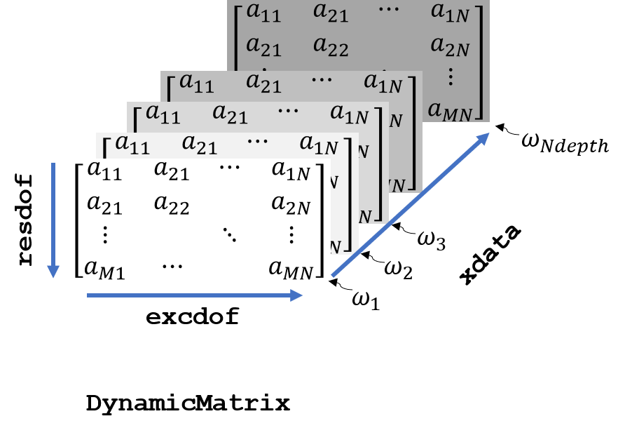
_images/DynMat.png — Sketch of DynamicMatrix.

To summarize, the main extension of DynamicMatrix to LinearMatrix is, that all dimensions of the three dimensional array are linked to either degrees of freedom of xdata, for example frequency as shown in figure Sketch of DynamicMatrix..

An example for a dynamic stiffness matrix is:

>>> u_dof = dof.DOF([1,2],[1,2,3],disp,repetition=True)
>>> f_dof = dof.DOF([1,2],[1,2,3],force,repetition=True)
>>> x_data = mC.DataAxis([10.,20.,30], typestr = 'angular frequency')
>>> data = data = 40*np.random.random_sample((6,6,3))

The DynamicMatrix is an extension of LinearMatrix, so all rules for the three-dimensional data apply for this class also:

>>> DD   = mC.DynamicMatrix(data, x_data, u_dof, f_dof)
>>> DD
LinearMatrix of size (6, 6, 3), sym: 0
DataAxis of 3 samples and type angular frequency in hertz
resdof: DOF object with ID [1 1 1 2 2 2], DOF [1 2 3 1 2 3] of type [force in newton]
excdof: DOF object with ID [1 1 1 2 2 2], DOF [1 2 3 1 2 3] of type [displacement in meter]

Many overloaded method of matrix operations can be used. The key feature is, that those methods take care about the degreed of freedom, too:

>>> DDinv = DD.inv()
>>> DDinv
LinearMatrix of size (6, 6, 3), sym: 0
DataAxis of 3 samples and type angular frequency in hertz
resdof: DOF object with ID [1 1 1 2 2 2], DOF [1 2 3 1 2 3] of type [displacement in meter]
excdof: DOF object with ID [1 1 1 2 2 2], DOF [1 2 3 1 2 3] of type [force in newton]

Note, that response and excitation degrees of freedom are now exchanged. Further multiplication with force excitation as load case provides the displacement response:

>>> f_data = np.zeros((6,3))
>>> f_data[1,:] = 1.
>>> force_load = mC.Signal(x_data,f_data, f_dof)

>>> u_res = DDinv.dot(force_load)
>>> u_res
Signal object of 3 samples with 6 channels and properties ...
DataAxis of 3 samples and type angular frequency in hertz
DOF object with ID [1 1 1 2 2 2], DOF [1 2 3 1 2 3] of type [displacement in meter]

Because of the internal degree of freedom logics it would be sufficient to create the load exclusively for the non zero components:

>>> f_data = np.ones((1,3))
>>> force_load = mC.Signal(x_data,f_data, f_dof[0])

The implemented dot() method applies the load only to the excited degree of freedom

>>> u_res = DDinv.dot(force_load)

With the same result as in the case before.