Hybrid FEM/SEA models

The creation and solution of hybrid models is a complex tasks including several steps. The reason for this is that two different model approaches are used that lead to a connection and an impact between and onto both disciplines.

The FEM parts that are connected to the SEA part influence the coupling between the SEA parts and may radiate additional power into the SEA systems. The SEA reverberant fields create an additional diffuse field excitation to the FEM systems that cause additional wave motion in the FEM systems.

The topic is too complex for the pyva documentation. Details are given in the original paper from Langley [Lan2005] or in [Pei2022].

The first example is similar to the two rooms example, but with a smaller plate as FEM system. In this case the impact of the FEM system is just a change of the coupling dynamics. The second example deals with a deterministic force excitation on the deterministic wall where a fully coupled approach of FEM and SEA is necessary. The global set-up for both cases is shown in the following figure

Two room configuration for hybrid cases.

The required import of this section are as follows:

import pyva.coupling.junctions as jun
import pyva.properties.structuralPropertyClasses as stPC
import pyva.systems.structure2Dsystems as st2Dsys
import pyva.systems.acoustic3Dsystems as ac3Dsys
import pyva.loads.loadCase as lC
import pyva.models as mds
import pyva.useful as uf
import pyva.data.dof as dof
import pyva.data.matrixClasses as mC
import pyva.properties.materialClasses as matC

The FEM subystem

Hybrid methods require a deterministic component in the system. This is usually the FEM part of those systems that are (still) deterministic.

In our case the FEM subsystem is generated or mapped from the analytical modal solutions. This is implemented in the FEM class pyva.models.FEM:

After populating the database

#Frequencies
omega_max = 2*np.pi*4000
omega = mC.DataAxis(np.geomspace(2*np.pi*25,omega_max,150), typestr = 'angular frequency')

# Plate dimensions
Lx = 0.8
Ly = 0.5

# Create material and propterty
alu    = matC.IsoMat(nu=0.3,eta = 0.0)
alu4mm = stPC.PlateProp(0.004,alu)

we create the rectangular plate system

plate = st2Dsys.RectangularPlate(2,Lx,Ly,prop=alu4mm,wave_DOF = [3],eta = 0.02)

as usual.

The FEM object is now created by mapping modes and defining a mesh with the normal_modes() method of the RectangularPlate class

# Create plate as FE-Model
modes,mesh = plate.normal_modes(omega_max*1.2,mapping = 'mesh')
plateFE    = mds.FEM(2,mesh,modes,damping_loss=0.02)

The modes are a Signal object. In the xdata attribute we find for example the angular modal frequencies

>>> plateFE.modes.xdata.data
array([  340.77343643,   627.94206263,  1075.92511951,  1106.55643964,
        1363.09374572,  1776.61656745,  1841.70812273,  ... ])

Two rooms with FE-plate

We populate the database and define the SEA systems

air = matC.Fluid()
room1 = ac3Dsys.Acoustic3DSystem(1, 64 , 96, 48, air)
room2 = ac3Dsys.Acoustic3DSystem(3, 80 ,112, 52, air, absorption_area = Lx* Ly, damping_type= ['surface'])

Note, that the absorption area of room 2 equals the plate surface to keep 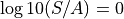. All systems are connected via a hybrid junction:

HJ123 = jun.HybridAreaJunction((room1,room2),plateFE)

The hybrid area junction assumes that the FEM system is centred between both cavities.

Sound source in room 1

We create a point power load in room1 with ID=1

power1Watt = lC.Load(omega, np.ones(omega.shape), dof.DOF(1,0,dof.DOFtype(typestr = 'power')), name = '1Watt')

The model is created by

# Create hybrid SEA model
RPR_SEA_exc = mds.HybridModel((room1,room2),FEsystems = (plateFE,),xdata=omega)
# connect and add load
RPR_SEA_exc.add_hybrid_junction({'HareaJ_12':HJ123})
RPR_SEA_exc.add_load('1Watt',power1Watt)

The solution will take some time, because the calculation of the modal radiation stiffnesses is computationally expensive.

RPR_SEA_exc.create_SEA_matrix(sym = 1)
RPR_SEA_exc.solve()

The energy result in both rooms is found in the results attribute and plotted by

RPR_SEA_exc.result.plot(4,ID=[1,3],xscale = 'log',yscale = 'log',
                   fulllegstr = ('room 1','room 2',))

Showing the typical spiky shape in the receiving room due to the plate resonances.

Pressure of the rooms.

The pressure fields in both rooms excite vibration on the FEM subsystem. There is a hybrid junction method that allows to calculate the response of the FEM systems in the junction

sqq_type = dof.DOFtype(typestr='displacement',exponent = 2)
# Determine CSPD of FEM system
Sqq_P = HJ123.FEM_response(omega.angular_frequency , RPR_SEA_exc.energy)
# Detrmine nodal average from modal response
x2rms_P,v_type = plateFE.rms_vec_from_modal_cpsq(Sqq_P,sqq_type = sqq_type)
# Convert into velocity
v2rms_P = (omega.angular_frequency*x2rms_P).flatten()

The following figure shown the rms response of the plate due to the reverberant loading from both rooms.

Root mean square velocity of plate.

For more details, especially regarding a comparison with SEA results please refer to [Pei2022]. Finally the TL follows directly from the squared pressure ratio.

p1 = RPR_SEA_exc.result[0].ydata.flatten()
p2 = RPR_SEA_exc.result[1].ydata.flatten()

tau = (p2/p1)**2

Transmission loss from hybrid model.

Force excitation at plate

In the second case a point force is exciting the plate. The global model is the same, but with a different load.

forceID = 199
force10N = lC.Load(omega, 10*np.sqrt(2)*np.ones(omega.shape), \
                          dof.DOF(forceID,3,dof.DOFtype(typestr = 'force')), \
                          name = '10N@Node'+str(forceID))
# check position
X,Y = mesh.nodes()
print('Excitation at X={0:.2f}, Y={1:.2f}'.format(X.flatten()[forceID],Y.flatten()[forceID]))

With output:

Excitation at X=0.31, Y=0.11

This force is deterministic and therefore added to the FE model and not the HybridModel.

plateFE.add_load(force10N)

We must tell the SEA solver to consider the response due to the deterministic load

RPR_FE_force.create_SEA_matrix(sym = 1,force = '10N@Node'+str(forceID))
RPR_FE_force.solve()

This provides the following figure derived from the result attribute.

Pressure of the rooms with plate force excitation.

The pressure becomes less in room 1 because the damping increases with frequency here, and decreases for the surface absorption in room 2. The radiated power is identical because the radiation efficiency into both rooms is similar. The response of the point force is stored in the hybrid_results attribute and plotted with:

RPR_FE_force.hybrid_result.plot(10,ID=2,xscale = 'log',yscale = 'log',fulllegstr = ['$S_{qq}$'])

The velocity response due to the reverberant fields ( so to say the effect of its own created sound) is recovered using the FEM_response method

sqq_type = dof.DOFtype(typestr='displacement',exponent = 2)
# Determine CSPD of FEM system
Sqq_F = HJ123.FEM_response(omega.angular_frequency , RPR_FE_force.energy)
# Determine nodal average from modal response
x2rms_F,v_type = plateFE.rms_vec_from_modal_cpsq(Sqq_F,sqq_type = sqq_type)
# Convert into velocity
v2rms_F = (omega.angular_frequency*x2rms_F).flatten()

The figure reveals that naturally the velocity due to the force is much higher than the vibration caused by the reverberant fields in the rooms.

Root mean square velocity of plate with force excitation.