Models module
The model classes are part of the models pyva.models module.
Global setup of a vibroacoustic model.
Finite Element Model (FEM)
In general, finite element models are the result of specific numerical method that models a structure or a fluid by subdividing the system into several finite elements. These methods are subject of many books, projects and research. In [Bat1982] a good overview about the method is for example given.
The current implementation of finite element models is very basic. Currently, only analytical mode shapes are mapped to two dimensional meshes in order to provide the modal database for the hybrid models.
A full scale FE-model comes with a mesh and coordinate system definition and the related mass and stiffness matrices that are required to determine the dynamic stiffness matrix for every frequency or to calculate the modal solutions. However, there is the intention to include this into later versions of pyva preferably from other packages that are already available.
Vibro Acoustic Model VAmodel
The VAmodel class pyva.models.VAmodel describes a deterministic system by a stiffness matrix for a given set of
degrees of freedom.
One typical example is given in equation (1).
(1)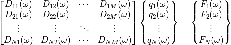
 are the coefficients of the dynamic stiffness matrix,
 the qeneralised displacement degrees of freedom and
 the generalized forces.
In FEmodels the mass and stiffness matrices are not frequency dependent.
In contrast to that, the dynamic stiffness matrix is frequency dependent matrix.
Naturally, the VAmodel class is an extension of the DynamicMatrix class with additional results and loads.
Many system classes from the systems module pyva.systems provide methods to generate entries into the matrix in
order to model such systems as part of a VAmodel.
For example the mass and stiffness matrices of an FE-model matrix equation can be converted into a dynamic stiffness representation by:
(2)
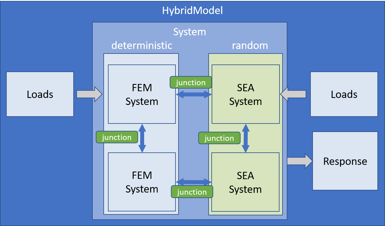
HybridModel
The HybridModel class pyva.models.HybridModel serves as a model container for SEA- and FEM-subsystems.
The subsystems can be connected via junctions and excited by specific loads.
The class attributes include SEA- and FEM-matrices that are required to calculate the
SEA and FEM response of the system.
The SEA part is given by the SEA matrix:
(3)
 are the coupling loss factors,
 the modal density of the wave system,
 the energy of the wave system and
 the input power.
Please note that only SEA Systems are obligatory. FEM-subsystems are not required, but can be included.
Transfer matrix model
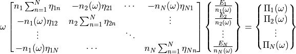
Sketch of connected infinite layers.
Especially the simulation of flat noise control treatment can be performed efficiently using the
transfer matrix method. The pyva.models.TMmodel class provides methods to deal with system configurations that can be
treated by transfer matrices.
Obviously, this is restricted to sequential arrangements, for example a series of tubes or infinite layers.
In figure Sketch of connected infinite layers. the arrangement of multiple layers, layer index n and node IDs used in the matrix set-up.
The convention in the node IDs is as follows; the wetting fluid layer is always index 0, every layer has two degrees of freedom an odd (left) and an even (right).
The node IDs are 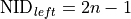 and
and 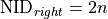 .
The potentially connected connected fluid has the
.
The potentially connected connected fluid has the 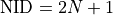 .
.
The advantage of the former pressure-velocity formulation was, that the dynamics of the full layer set-up could be calculated by a simple chained matrix multiplication of all transfer matrices. With the new mix of layers of different nature this is no longer possible. Now, specific interface conditions are required making the calculation of the dynamics much more complicated.
However, when the physics and the nature of the layer is not changed the transfer matrix multiplication can still be used - except for poroelastic layers that requires the consideration of different porosities.
The Allard matrix
The sound transmission of a specific layer set is performed solving a complex matrix that takes the different wave propagation, the coupling between the layers and the boundary conditions into account. This is namely the matrix of equation (11.79) of [All2009] with the extra lines of equation (11.82) for hard wall termination or (11.84) and (11.85) for the free field. The excitation is given by equation (11.86) which makes the final matrix square.
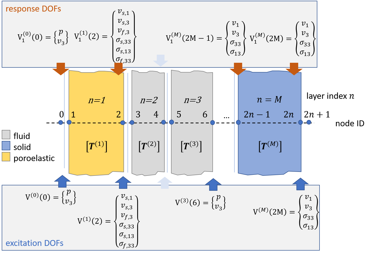
Logics of response and excitation DOFs of multiple infinite layers.
The Allard matrix is implemented as a DynamicMatrix object. The exc_DOF correspond exactly to the  vector of Allard.
In order to explain the logics of the DynamicMatrix creation we consider the equation that constitute the dynamics for the right degrees of freedom of specific layers, namely (11.69) of [All2009].
vector of Allard.
In order to explain the logics of the DynamicMatrix creation we consider the equation that constitute the dynamics for the right degrees of freedom of specific layers, namely (11.69) of [All2009].
(4)
The numbers in the argument parenthesis of  are the node ID, the upper index in round parenthesis is the layer.
The transfer matrix is the reason why only the right node IDs are taken as exc_dof. In contrast to Allards equation we skip the internal node IDs when layers of similar nature are connected.
In this case (and neglecting the porous-porous connection) the equation would read as:
are the node ID, the upper index in round parenthesis is the layer.
The transfer matrix is the reason why only the right node IDs are taken as exc_dof. In contrast to Allards equation we skip the internal node IDs when layers of similar nature are connected.
In this case (and neglecting the porous-porous connection) the equation would read as:
(5)
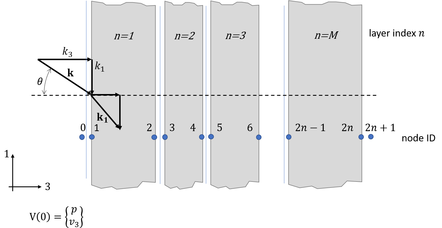
A final matrix might look like.
(6)![\begin{bmatrix}
{\bm D}_0
\end{bmatrix}
\begin{bmatrix}
[I_{f1}] & [J_{f1}][T^{(1)}] & [0] & \cdots & [0] & [0] \\
[0] & [I_{12}] & [J_{12}][T^{(2)}][T^{(3)}] & \cdots & [0] & [0] \\
\vdots & \vdots & \vdots & & \vdots & \\
[0] & [0] & [0] & \cdots & [J_{(M-2)(M-1)}][T^{(M-1)}] & [0] \\
[0] & [0] & [0] & \cdots & [J_{(M-1)(M)}] & [I_{(M-1)(M)}][T^{(M)}]
\end{bmatrix}](_images/math/b8b8faf01080c8078b916f6facff623dc00eadbc.png)
And the exc_dof
(7)
The res_dof is vector of response degrees of freedom according to the discussions of section sec-coupling-TM. Depending on the end boundary conditoin there may be additoinal degrees of freedom added. We check the procedure using an example starting with the import of required libraries.:
import pyva.models as mds
import pyva.systems.infiniteLayers as iL
import pyva.properties.structuralPropertyClasses as stPC
import pyva.properties.materialClasses as matC
Next we create all materials and properties:
# Fluids
air = matC.Fluid(air)
poro_limp = matC.EquivalentFluid(rho_bulk = 30., \
                                flow_res = 40000., \
                                porosity = 0.94, \
                                tortuosity = 1.06, \
                                length_visc = 56.E-6, length_therm = 110.E-6,limp=True)
# Poroelastic
ela_vac = matC.IsoMat(4400000.0,130., 0., 0.1) # Frame in vaccuum
poroela = matC.PoroElasticMat(ela_vac, \
                            flow_res = 40000., \
                            porosity = 0.94, \
                            tortuosity = 1.06, \
                            length_visc = 56.E-6, length_therm = 110.E-6)

# Solid
alu = matC.IsoMat()
alu1mm = stPC.PlateProp(0.001,alu)
and create infinite Layers of them
# Layers
il_alu_solid_1mm = iL.SolidLayer(alu1mm,)
il_air_10mm      = iL.FluidLayer(0.01,fluid=air)
il_fibre_20mm    = iL.FluidLayer(0.02,fluid=poro_limp)
il_poro_ela      = iL.PoroElasticLayer(poroela, 0.05)
Finally a TMmodel object is create from these layers:
TM_all = mds.TMmodel((il_poro_ela,il_air_10mm,il_fibre_20mm,il_alu_solid_1mm))
The configuration fits quite well to figure Logics of response and excitation DOFs of multiple infinite layers.. Note that the
second and third layer are fluid layer so the DOFs in the middle.
With the V0() method the excitation and response DOFs are derived:
V0,V1 = TM_all.V0()
>>>V0DOF object with ID [0 0 2 2 2 2 2 2 6 6 8 8 8 8 9 9], DOF [0 3 1 3 2 3 5 2 0 3 1 3 3 5 0 3] of type
[DOFtype(typestr='pressure'), DOFtype(typestr='velocity'), DOFtype(typestr='velocity'), ... ]
See the node IDs 0 2 6 8 and 9 of the exc_DOF. Node 4 is skipped because of the two fluid layers. The 9 comes from the final layer that is assumed as fluid or half space end condition. See also the different DOFs of the V0 vector. The res_dof is different as discussed before:
>>>V1
DOF object with ID [1 1 1 1 2 2 2 2 7 7 7 8 8 8 9], DOF [1 3 5 2 1 3 5 2 3 3 1 3 3 1 0] of type
[DOFtype(typestr='velocity'), DOFtype(typestr='stress'), DOFtype(typestr='stress'), ... ]
The res_dof vector has lower size and the node ID is linked to the complicated part of the interface. This is node 1 or the first poroelastic layer and node 7 of the lase solid layer.
The full Allard matrix is calculated using the allard_matrix() method:
D0 = TM_all.allard_matrix(6000., kx = 0.,reduced = False)
This matrix is solved by setting the excitation pressure at node ID 0 to 1, eliminate the first coloumn and row of the
matrix and create a force vector of it. This is requested by the reduced = True keyword argument:
D1,F = TM_all.allard_matrix(6000., kx = 0.,reduced = True)
The response in all DOFs can be calculated using the pyva.data.matrixClasses.DynamicMatrix.solve() method of
the DynamicMatrix
Vs = D1.solve(F)
This functionality is used in the transmission_allard() and
impedance_allard() method.