SEA models
In Statistical Energy Analysis the vibroacoustic system is modelled as systems of coupled reverberant wave fields that exchange energy. The method is described in in [Lyo1995] and [Pei2022] in detail or briefly in SEA introduction. For the set-up of such models the database must be populated with system properties namely the geometry, the property determining the wave motion, the coupling physics and the sources.
Required imports
The examples in this section require the import of the models module and further modules from subpackages.
Thus, we start with the following import commands:
# Other modules
import numpy as np
import matplotlib.pyplot as plt

# pyva modules
import pyva.models as mds

# coupling
import pyva.coupling.junctions as con

# systems and loads
import pyva.systems.structure2Dsystems as st2Dsys
import pyva.systems.acoustic3Dsystems as ac3Dsys
import pyva.loads.loadCase as lC

# properties
import pyva.properties.structuralPropertyClasses as stPC
import pyva.properties.materialClasses as matC

# data classes
import pyva.data.dof as dof
import pyva.data.matrixClasses as mC

# useful things
import pyva.useful as uf
Two rooms separated by a wall
This building acoustic example deals with two rooms that are separated by a concrete wall. The configuration is shown in figure Two rooms separated by a concrete wall..

Two rooms separated by a concrete wall.
We start with the material properties and use typical data for air and light concrete:
h        = 0.05           # wall thickness
air      = matC.Fluid()   # default air
concrete = matC.IsoMat(E=3.8e9,nu=0.33,rho0=1250.)
The wall has thickness 5 cm thus:
concrete_5cm = stPC.PlateProp(h,concrete)
Due to the fact that the setup is rectangular we use the rectangular versions of system description:
# wall dimensions
Ly = 4.
Lz = 2.5
S  = Lz*Ly

# Additional room dimensions
Lx1 = 3.
Lx2 = 5.
# Absorption area
As1  = 8.
As2  = 10.

wall  = st2Dsys.RectangularPlate(2, Ly,Lz,prop=concrete_5cm, eta = 0.03)
room1 = ac3Dsys.RectangularRoom(1, Lx1, Ly, Lz, air, absorption_area = As1, damping_type= ['surface'])
room2 = ac3Dsys.RectangularRoom(3, Lx2, Ly, Lz, air, absorption_area = As2, damping_type= ['surface'])
The damping_type argument assures that the air damping is not used but only damping from surface absorption.
The logical next step is to couple all systems by an AreaJunction.
If no area argument is given the coupling surface defaults to the surface of the wall:
J123 = con.AreaJunction((room1,wall,room2))
The centre system must be the wall if three systems are involved.
In addition, the frequency range must be defined. This is usually a third-octave band spectrum in SEA and building acoustics.
omega = mC.DataAxis.octave_band(f_max=2*np.pi*10000)
Helper variables are created in addition for easier plotting of the frequency axis in Hertz:
om    = omega.data
freq  = om/2/np.pi
One source is assumed to introduce power into the first room. This load is defined by:
pow_dof     = dof.DOF(1,0,dof.DOFtype(typestr = 'power'))
power1mWatt = lC.Load(omega, 0.001*np.ones(omega.shape), pow_dof, name = '1mWatt')
We have collected all input to create the model using the HybridModel class but without FEM systems included
two_rooms = mds.HybridModel((wall,room1,room2),xdata=omega)
two_rooms.add_junction({'areaJ_12':J123})
two_rooms.add_load('1mWatt',power1mWatt)
and solve it:
two_rooms.create_SEA_matrix()
two_rooms.solve()
The next step is to work with the model, query some details and access the result. We start with the evaluation of the random properties and take a deeper look on the modal density
plt.plot(freq,wall.modal_density(om,3),label = 'wall')
plt.plot(freq,wall.modal_density(om,5),label = 'wall')
plt.plot(freq,room1.modal_density(om),label = 'room1')
plt.plot(freq,room2.modal_density(om),label = 'room2')
With the following result:

Modal density of SEA systems.
Of further importance is the modal overlap:
plt.plot(freq,wall.modal_overlap(om,3),label = 'wall') ...
plt.plot(freq,wall.modal_overlap(om,5),label = 'wall') ...
plt.plot(freq,room1.modal_overlap(om),label = 'room1')
plt.plot(freq,room2.modal_overlap(om),label = 'room2')
leading to:

Modal overlap of SEA systems.
Note that the modal overlap is larger than 1 for all frequencies, except for the combined in plane waves (LS). Due to their high sound speed the modal overlap becomes high enough above 1kHz.
For better understanding of the coupling dynamics it is helpful to investigate the radiation
physics of the wall. The coincidence frequency is a method of the
PlateProp class:
f_c = concrete_5cm.coincidence_frequency(air.c0)/2/np.pi
>>> f_c
702.353
So, this wall will have critical sound isolation properties at 700 Hz (which is not a good design for buildings). For the wall system we can derive the radiation efficiency in two ways:
sigma        = wall.radiation_efficiency(om,fluid = air)
sigma_simple = wall.radiation_efficiency_simple(om,fluid = air)
The first method uses Leppingtons simplified approach [Lep1982] averaged over the quarter wavenumber circle, the second method is an implementation of the ISO EN 12354-1.
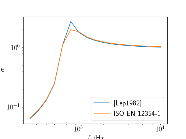
Radiation efficiency of the wall derived by different methods.
Both methods agree well except in the coincidence peak. See [Pei2022] for details of the implementation.
Next, the SEA results are investigated in detail. In general the result of each [All2009]s are of class Signal.
The solution generate results in the energy and result attribute :
>>> two_rooms.energy
Signal object of 17 samples with 4 channels and properties ...
DataAxis of 17 samples and type angular frequency in 1 / second
DOF object with ID [2 2 1 3], DOF [3 5 0 0] of type [energy in joule]
Thus the methods from the Signal class can be used for plotting and further query. Starting with the energy of each system / wavefield:
two_rooms.energy.plot(20,xscale = 'log',yscale = 'log',ls = ['-','--',':','-.'],
        fulllegstr = ('wall B','wall LS','room1','room2'))

Energy of subsystems.
Note that there is no energy in the LS wavefield because it is not coupled to the room acoustic wave field.
For, all systems the engineering unit was also calculated automatically:
>>> two_rooms.result
Signal object of 17 samples with 4 channels and properties ...
DataAxis of 17 samples and type angular frequency in 1 / second
DOF object with ID [2 2 1 3], DOF [3 5 0 0] of type [velocity in meter / second, velocity in meter / second, pressure in pascal, pressure in pascal]

Velocity of the wall.

Pressure of the rooms.
For the determination of the acoustic performance of the wall we calculate the transmission loss.
Because of  [Pei2022] the transmission coefficient can be calculated directly from the
pressure ratio of both rooms.
[Pei2022] the transmission coefficient can be calculated directly from the
pressure ratio of both rooms.
p1 = two_rooms.result[2].ydata.flatten()
p2 = two_rooms.result[3].ydata.flatten()
tau = (p2/p1)**2
TL = -10*np.log10(tau)
The transmission loss in figure Transmission loss of the wall clearly reveals the coincidence dip.

Transmission loss of the wall
Further insight is provided when the power inputs to room2 are calculated, revealling that the power radiated from the wall is dominating over a large frequency range
pow_in_room1 = two_rooms.power_input(3)

Power input to room 2
Two rooms with floor separated by a wall
The first case is a pure airborne transmission case. A more realistic example is created by adding a floor to both rooms.
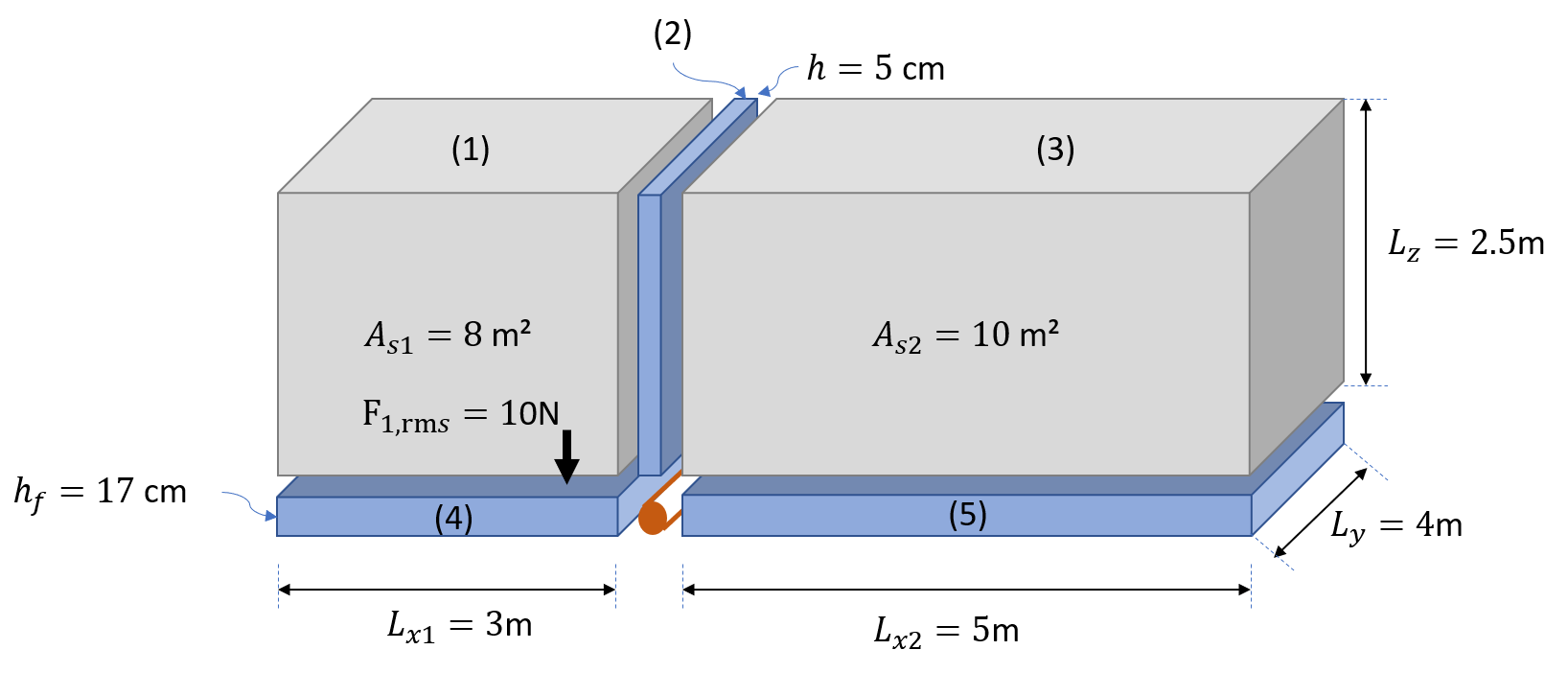
Two rooms separated by a concrete wall plus floor plates.
The floor is supposed to have higher thickness than the wall
concrete_17cm = stPC.PlateProp(h_f,concrete)
and the floor subsystems have ID=4 and 5
floor1 = st2Dsys.RectangularPlate(4, Lx1,Ly,prop=concrete_17cm, eta = 0.03)
floor2 = st2Dsys.RectangularPlate(5, Lx2,Ly,prop=concrete_17cm, eta = 0.03)
Both floor are connected to the rooms by area junctions
J14  = con.AreaJunction((room1,floor1))
J35  = con.AreaJunction((room2,floor2))
The ‘T’-connection of both floor plates and the wall is a LineJunction of length Ly
J425 = con.LineJunction((floor1,wall,floor2),length = Ly, thetas = (0,90,180))
Instead of the power source in room1 a force excitation at floor1 is used
force10Nrms = lC.Load(omega, 10*np.ones(omega.shape), dof.DOF(4,3,dof.DOFtype(typestr = 'force')), name = '10N')
The DOF instance determines the excitation at system ID=4 (floor1) and wave_DOF=3 (bending). The model is created by
omega = mC.DataAxis.octave_band(f_min=2*np.pi*50,f_max=2*np.pi*10000)

two_rooms = mds.HybridModel((wall,room1,room2,floor1,floor2),xdata=omega)
with the junctions and load defined by
two_rooms.add_junction({'areaJ_123':J123})
two_rooms.add_junction({'areaJ_14':J14})
two_rooms.add_junction({'areaJ_35':J35})
two_rooms.add_junction({'lineJ_425':J425})

two_rooms.add_load('10N',force10Nrms)# add force excitatio to wave_DOF 3 of system 4
The frequency starts at 50Hz for illustrating some typical checks in SEA [All2009]. Before, we solve the model we perform these typical checks. This time the modes in band of the plate systems are shown in the following figure:

Modes in band of plate subsystems.
One rule of thumb of SEA is, that a subsystem should have at least 5 modes in band. This is the case for all subsystems above 400 Hz. Results at lower frequencies should be considered as not very precise. However, due to higher thickness of the floor the coincidence frequency is lower than for the wall
f_cf = concrete_17cm.coincidence_frequency(air.c0)/2/np.pi
>>> f_cf
206.57440
So, the coincidence frequency is at 200 Hz and the floor plates will be good radiators for the full SEA frequency range. The radiation efficiency of both floor plates is shown in the following figure:

Radiation efficiency of floor plates.
The force excitation on floor 1 radiates acoustic power into all wave field. the line junction transfers energy from the bending wave field into the in-plane (LS) wave field.

Energy of subsystem wave field due to 10N rms excitation. When converted into the engineering results. the pressure and velocity results read as follows:
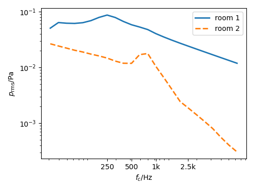
Pressure result of rooms.

Bending wave field velocity.
The pressure in room 1 shows a coincidence peak at the floor coincidence. So the floor1 is the main
radiator for room 1. Room 2 has the coincidence peak at wall coincidence.
In order to determine the dominant path we apply the pyva.models.HybridModel.power_input() method:
pow_in_room1.plot(32,yscale = 'log',xscale = 'log')
pow_in_room2.plot(32,yscale = 'log',xscale = 'log')
The curves in figure Power input to room 1. reveal that the main power input comes from the radiating floor1 and wall that has received acoustic energy from the line junction. In figure Power input to room 2. the situation is different. Here, the wall bending wave is the main source of energy followed by the floor 2 wave. Non resonant air transmission from room 1 contributes least.
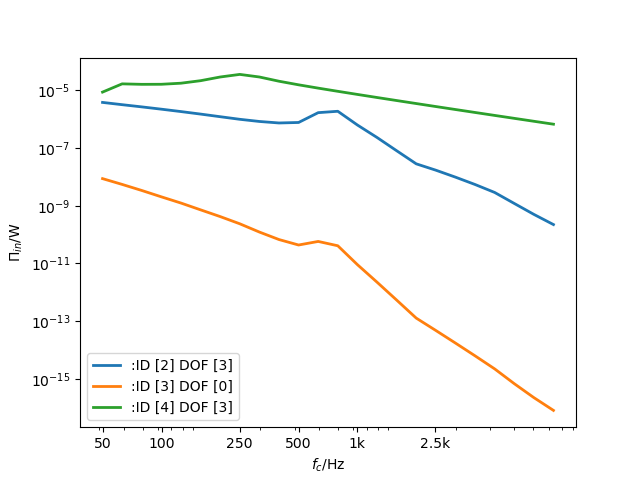
Power input to room 1.

Power input to room 2.
Box cover of sound source
The next example shows an application of box structures for sound isolation.
In addition it is an application of the SemiInfiniteFluid class of the junctions module
and it illustrates
the limit of text based model description. Due to the large number of junction and systems
even for such a simple box it becomes clear that for later complex model applications a GUI and
a 3D representation of the models will be mandatory.
The set-up is shown in the following figure
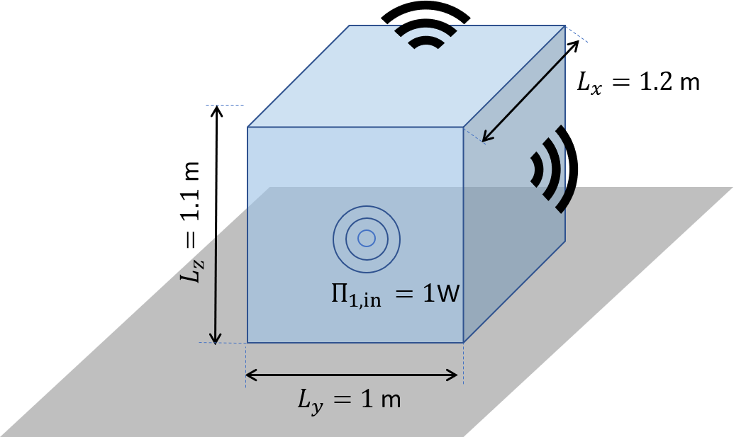
SEA model of box covering a power source
First, we define the frequency range and the box dimensions:
# Frequency range
omega = mC.DataAxis.octave_band(f_max=2*np.pi*10000)

# Plate dimensions
Lx = 1.2
Ly = 1
Lz = 1.1

# Box dimensions
V = Lx*Ly*Lz
A = 2*(Lx*Ly+Ly*Lz+Lx*Lz)
P = 4*(Lx+Ly+Lz)

# Plates thickness
t = 2.0E-3;

# junction angle
angle_R = (0.,90*np.pi/180)
and the materials and properties
# Create materials
steel = matC.IsoMat(E=210e9,nu=0.3,rho0=7800, eta = 0.0)
air   = matC.Fluid()

# Create props
steel2mm = stPC.PlateProp(t,steel)
Next step is the creation of the subsystems
# Create plate subsystems
plate1 = st2Dsys.RectangularPlate(1,Lx,Lz,prop = steel2mm)
plate2 = st2Dsys.RectangularPlate(2,Ly,Lz,prop = steel2mm)
plate3 = st2Dsys.RectangularPlate(3,Lx,Lz,prop = steel2mm)
plate4 = st2Dsys.RectangularPlate(4,Ly,Lz,prop = steel2mm)
plate5 = st2Dsys.RectangularPlate(5,Lx,Ly,prop = steel2mm)

room     = ac3Dsys.Acoustic3DSystem(6, V , A, P, air)
The box is emerged in free space and requires semi infinite fluid (SIF) to allow free space radiation. SIFs are created by a list of connected subsystems (where the connection can be resonant and non-resonant) and the fluid into which the radiation takes place.
# create semi infinite fluids
sif1 = jun.SemiInfiniteFluid((room,plate1), air)
sif2 = jun.SemiInfiniteFluid((room,plate2), air)
...
All junctions are here created as dictionary from scratch.
juncs =  { 'j61' : jun.AreaJunction((room,plate1)),
           'j62' : jun.AreaJunction((room,plate2)),
           ...
           'j12' : jun.LineJunction((plate1,plate2), Lz, angle_R),
           'j23' : jun.LineJunction((plate2,plate3), Lz, angle_R),
            ... }
Not to forget the power source in the room (ID = 6)
power1W = lC.Load(omega, np.ones(omega.shape), dof.DOF(6,0,dof.DOFtype(typestr = 'power')), name = '1Watt')
Finally we create the model and put things together
#create SEA model
box = mds.HybridModel((plate1,plate2,plate3,plate4,plate5,room),xdata=omega)

#connect all
box.add_junction(juncs)
box.add_SIF({'sif1' : sif1,
             'sif2' : sif2,
             'sif3' : sif3,
             'sif4' : sif4,
             'sif5' : sif5})

box.add_load('1Watt',power1Watt) # add 1Watt per band
and solve it
box.create_SEA_matrix(sym = 1)
box.solve()
The interesting feature here is how much of the power is removed from the source. With the
pyva.models.HybridModel.power_input() method, we get the power inputs into the SIFs
sif1_in = box.power_input('sif1')
sif2_in = box.power_input('sif2')
sif3_in = box.power_input('sif3')
sif4_in = box.power_input('sif4')
sif5_in = box.power_input('sif5')
Plotting the result for example for SIF1 we see the non-resonant (ID=6) and resonant (ID=3) power radiation to the free space.

Input power to SIF1
All values are added by using the sum() method of Signal
that add all those paths in one signal and adding all SIF contributions:
sif_all = sif1_in.sum()+sif2_in.sum()+sif3_in.sum()+sif4_in.sum()+sif5_in.sum()
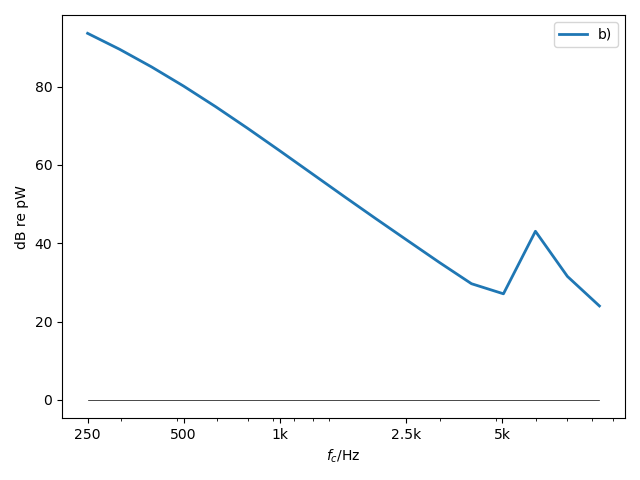
This leads to the total source level

Total input power to all SIFs
Note that 1Watt corresponds to Lw=120 dB, so noise reduction is not perfect.
Box cover with noise control treatment
Typical noise control strategy would start at the source. Let’s say that this is not possible here, so the next step is first to bring absorption into the cavity and second to increase the isolation by an extra treatment. The configuration from the last section a) and this one b) is shown in the following figure.

Pure and trimmed configuration
We create the additional materials and properties for the treatment
import pyva.systems.infiniteLayers as iL

# Fibre material
rho_bulk = 0.98*1.20 + 30.
fibre1 = matC.EquivalentFluid(porosity = 0.98, \
                               flow_res = 25000.,\
                               tortuosity = 1.02, \
                               length_visc = 90.e-6, \
                               length_therm = 180.e-6,\
                               rho_bulk = rho_bulk , \
                               rho0 = 1.208, \
                               dynamic_viscosity = 1.81e-5 )

# Thickness of fibre layer
h1 = 0.05
From those properties, infinite layer are created
fibre_5cm = iL.FluidLayer(h1,fibre1)
heavy_1kg = iL.MassLayer(0.001, 1000)
The treatments are defined via the TMmodel class
nct_mass     = mds.TMmodel((fibre_5cm,heavy_1kg))
nct          = mds.TMmodel((fibre_5cm,))
As the absorption is always determined at the (left) layer interface, we must reverse the treatment for the absorption determination
nct_mass4abs = mds.TMmodel((heavy_1kg,fibre_5cm))
For the box cavity absorption we use the absorption_diffuse method
# absorption due to trim
alpha_nct      = nct.absorption_diffuse(om,in_fluid=air)
alpha_nct_mass = nct_mass4abs.absorption_diffuse(om,in_fluid=air)
The abs_area is created from the specifically treated areas
abs_area = alpha_nct*(Lx*Ly)+alpha_nct_mass*(A-Lx*Ly)
# This is a signal those dof must be set to the area DOF
abs_area.dof = area_dof
The absorption area is not constant and therefore a Signal:
abs_area.plot(1,xscale = 'log')
This leads to a figure that shows that at high frequencies the absorption at the floor plate area of 1.2m^2 is dominant.

Absorption area due to NCT
To make the NCT working we add it to the plate systems and the absorption area to the room
# Create plate subsystems
plate1 = st2Dsys.RectangularPlate(1,Lx,Lz,prop = steel2mm,trim=(nct_mass,'none'))
plate2 ...

room   = ac3Dsys.Acoustic3DSystem(6, V , A, P, air,\
                        absorption_area = abs_area ,\
                        damping_type= ['eta','surface'] )
The value to the damping_type keyword parameter tells pyva that both damping effects are used.
This adds the absorption to the cavity and increases the isolation due to the mass-spring treatment leading
to a much higher isolation and lower sound power levels.
Total input power to all SIFs for isolated box.
Price and Crocker double panel transmission loss using SEA
The first simulation of the sound transmission of double wall panels was given by Price and Crocker [Pri1970]. In this paper all resonant and non-resonant path is dealt with, but neglecting the deterministic nature of this set-up and the strong coupling at the double wall resonance. Pyva is an excellent tool to study the details of the models of this paper. A detailed description is found in price example on my author page. The full code is given in Price and Crocker double panel transmission loss using SEA.
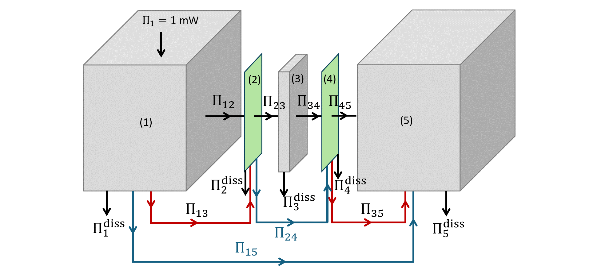
Possible paths of the double panel set-up from [Pri1970] in the paper version presenting both power flows in one arrow