Infinite Layers

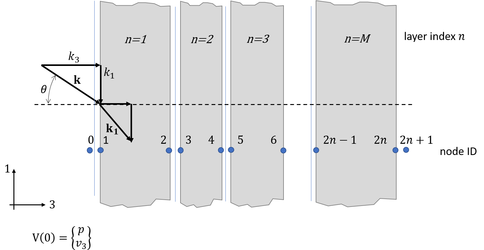
_images/infinite_layer.png — Sketch of connected infinite layers.

The infinite layer module models one dimensional systems as presented for example in the acoustic1Dsystems module. But here the dimensions perpendicular to the propagation direction are assumed to be infinitely extended instead of cross-sections with dimensions smaller than the wavelength. Consequently, there is an additional parameter required to deal with the infinite dimension: the in-plane wavenumber. For $k_1=0$ we have the same case as for one dimensional systems.

Lay-ups of practical interest may contain layers of various nature. According to Allard [All2009] this could be:

Foams or poro elastic materials
Fibre materials
Thick solid layers
Plate layers called impervious layers
Perforates

Due to the different nature of the layers, different degrees of freedom are required to describe the wave propagation. In a first version of pyva all layers could be modelled using pressure and out-of-plane velocity as degrees of freedom. With the introduction of new layers and physics this has changed.

Infinite layers are used as system in the pyva.models.TMmodel class. This class provides the framework for combining these layers and calculating global properties as absorption of transmission coefficients. See section TMM - infinite Layer for applications of infinite layer in transfer matrix models.

Acoustic Layer

All infinite layer classes are subclasses of the pyva.systems.infiniteLayers.AcousticLayer. This class is an abstract class that implements all those methods that required by all infinite layers. The subclass assumes the simplest case of degrees of freedom pressure and velocity. In [All2009] the acoustic layers are called fluid layer because they can be described using the degrees of freedom of a fluid.

(1) ${\bm V}_i = \begin{Bmatrix} {\bm p} \\ {\bm v}_3 \end{Bmatrix}$

The related DOF object is created by the fluid_exc_dof() function.

Beside the constructor that is exclusively used by the subclasses there is the get_xdata() method that implements a specific logics for the wavenumber and angular frequency argument.

Mass Layer

The simplest AcousticLayer is the MassLayer. As all subclasses it has implemented the transfer_impedance method that provides the 2x2 DynamicMatrix of the following form.

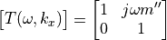
(2) $\begin{bmatrix} T(\omega,k_x) \end{bmatrix} = \begin{bmatrix} 1 & j\omega m'' \\ 0 & 1 \end{bmatrix}$

$m''$ mass per area

The muss layer does not depend on the wavenumber. As the so called mass law of transmission is quite important in acoustics it is implemented for this class.

import pyva.systems.infiniteLayers as iL
heavy_2kg7 = iL.MassLayer(0.001, 2700)

tau_mass0  = heavy_2kg7.transmission_coefficient(omega,0.)
tau_mass30 = heavy_2kg7.transmission_coefficient(omega,30.*np.pi/180)

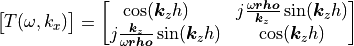
Plate Layer

When the plate is modelled as AcousticLayer there is connection of motion in in-plane direction considered. In other words every layer is free in x-direction.

The above matrix implements a different transfer impedance

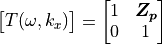
(3) $\begin{bmatrix} T(\omega,k_x) \end{bmatrix} = \begin{bmatrix} 1 & \bm{Z_p}\\ 0 & 1 \end{bmatrix}$

With $\bm{Z_p}$ as transfer impedance of flat plates.

A plate is defined as follows.

import pyva.properties.structuralPropertyClasses as stPC
alu = matC.IsoMat()
alu1mm = stPC.PlateProp(0.001,alu)
iL_alu1mm = iL.PlateLayer(alu1mm,)

The PlateLayer class comes also with the transmission coefficient method

tau_plate0  = iL_alu1mm.transmission_coefficient(omega,0.)
tau_plate30 = iL_alu1mm.transmission_coefficient(omega,30.*np.pi/180)

Plotting all curves gives the typical infinite behaviour with the sharp coincidence.

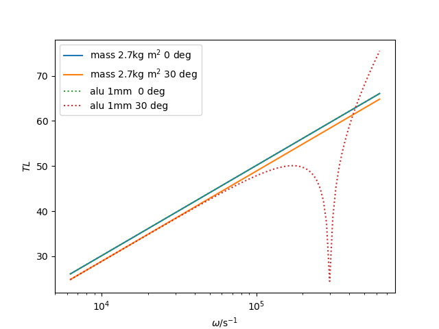
_images/infinite_layer_TL.png — Transmission loss of mass- and plate layer of same area weight

Fluid Layer

An air gap or a layer of material that can be modelled as EquivalentFluid is implemented as FluidLayer. The transfer matrix of such a layer with complex wavenumber $\bm{k}$ and thickness $h$ reads.

(4) $\begin{bmatrix} T(\omega,k_x) \end{bmatrix} = \begin{bmatrix} \cos(\bm{k}_{z} h) \quad & j \frac{\omega\bm{rho}}{\bm{k}_{z}} \sin(\bm{k}_{z} h) \\ j \frac{\bm{k}_{z}}{\omega\bm{rho}} \sin(\bm{k}_{z} h) & \cos(\bm{k}_{z} h) \end{bmatrix}$

This result follows from two fluid waves propagating in positive and negative direction with 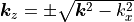$\bm{k}_z=\pm\sqrt{\bm{k}^2-k_x^2}$ and given $k_x$ . Details of the derivation are given in section 9.3.3 of [Pei2022].

Fluid Layer Honeycomb

The honeycomb channels restrict the direction of propagation to pure z-propagation. Thus, in case of a honeycomb layer equation fluid-transfer-matrix is used with $k_x=0$ .

Solid Layer

The physics of the solid layer of isotropic solids is similar to the PlateLayer but instead of using in-plane and out-of_plane waves (bending) for the description, the layer is modelled by longitudinal- and shear-waves. Hence, there are two waves propagating in two directions. Consequently the degrees of freedom that are required to describe the wave propagation are velocity in x- and z-direction as far as two coefficients of the stress tensor.

(5) ${\bm V}_i = \begin{Bmatrix} {\bm v}_1 \\ {\bm v}_3 \\ {\bm \sigma}_{33} \\ {\bm \sigma}_{13} \\ \end{Bmatrix}$

Please note, that the 13 index means index 5 in Voigt notation. Thus, this is 5 for local DOF orientation in the DOF class, meaning the rotation around the y-axis. So, we leave the practical world of similar degrees of freedom for each layer. As for all layers it is assumed that there is no propagation in y-direction.

The related DOF object is created by the solid_exc_dof() function.

The detailed matrices are too detailed to be presented here, but the theory is presented in [All2009] in detail. However, the formulas have some typos and cannot be implemented as is. However, a correct formula for the solid layer is given in Appendix A of [Ara2021].

Bending waves are automatically included by this approach. So, the solid layer can be considered as a thick layer implementation of the plate.

In addition the effect of the solid layer in the full lay-up is different. By defining the velocity and shear stress in x-direction. A solid layer restricts the x-degrees of freedom of the connected layer.

Impervious Screen

The impervious screen is a different implementation of the sec:plate_layer. In contrast to the plate the impervious screen has the degrees of freedom of the solid layer. So there is an in-plane motion, but the velocity in x- and z-direction is equal on both sides.

The transfer matrix reads:

(6) $[\bm T]_i = \begin{bmatrix} 1 & 0 & 0 & 0 \\ 0 & 1 & 0 & 0 \\ 0 & -{\bm Z}_p & 1 & 0 \\ -{\bm Z}_s & 0 & 0 & 1 \end{bmatrix}$

Here, ${\bm Z}_p$ is the same as in equation plate-transfer-matrix. ${\bm Z}_s$ is the in-plane impedance and read as.

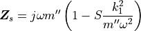
(7) ${\bm Z}_s = j\omega m'' \left(1-S \frac{k_1^2}{m''\omega^2}\right)$

With $S$ beeing the transversal stiffness implemented in S_complex().

Poroelastic Layer

The physics of the poroelastic layer is a combination of fluid motion (in the porous material) and the structure motion of the frame. Thus, the combination of required degrees of freedom becomes quite complex.

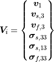
(8) ${\bm V}_i = \begin{Bmatrix} {\bm v}_1 \\ {\bm v}_{s,3} \\ {\bm v}_{f,3} \\ {\bm \sigma}_{s,33} \\ {\bm \sigma}_{s,13} \\ {\bm \sigma}_{f,33} \\ \end{Bmatrix}$

Because of the fact that we have the similar degree of freedom for the fluid and the structure in two cases, namely the velocity and stress in z-direction a work around is required. Thus, the local DOF of 2 is taken for the fluid DOF - please keep this in mind as it is not the real orientation.

The related DOF object is created by the porous_exc_dof() function.

The detailed matrices are definitely too detailed to be presented here, but the theory is presented in [All2009] in detail. To my surprise, these formulas have no typos and can be implemented as is.

In pyva the transfer matrix is calculated using the coordinate change of the Gamma function, thus:

(9) $\begin{bmatrix} {\bm T}_n \end{bmatrix} = \begin{bmatrix} {\bm \Gamma}(-h) \end{bmatrix} \begin{bmatrix} {\bm \Gamma}(0) \end{bmatrix}^{-1}$

The Gamma matrix can be found in [All2009] and the inversion is done analytically with the following result:

(10) $\begin{bmatrix} {\bm \Gamma}(0) \end{bmatrix}^{-1} = \begin{bmatrix} \frac{2 E_{2} N k_{1}}{\omega \left(D_{1} E_{2} - D_{2} E_{1} - 2 E_{1} N k_{1}^{2} + 2 E_{2} N k_{1}^{2}\right)} & 0 & 0 & \frac{E_{2}}{- D_{1} E_{2} + D_{2} E_{1} + 2 E_{1} N k_{1}^{2} - 2 E_{2} N k_{1}^{2}} & 0 & \frac{D_{2} + 2 N k_{1}^{2}}{D_{1} E_{2} - D_{2} E_{1} - 2 E_{1} N k_{1}^{2} + 2 E_{2} N k_{1}^{2}}\\ 0 & \frac{k_{1}^{2} \mu_{2} - 2 k_{1}^{2} \mu_{3} - k_{33}^{2} \mu_{2}} {k_{13} \omega \left(k_{1}^{2} \mu_{1} - k_{1}^{2} \mu_{2} + k_{33}^{2} \mu_{1} - k_{33}^{2} \mu_{2}\right)} & \frac{1}{k_{13} \omega \left(\mu_{1} - \mu_{2}\right)} & 0 & \frac{k_{1} \left(\mu_{2} - \mu_{3}\right)}{N k_{13} \left(k_{1}^{2} \mu_{1} - k_{1}^{2} \mu_{2} + k_{33}^{2} \mu_{1} - k_{33}^{2} \mu_{2}\right)} & 0\\ \frac{2 E_{1} N k_{1}}{\omega \left(- D_{1} E_{2} + D_{2} E_{1} + 2 E_{1} N k_{1}^{2} - 2 E_{2} N k_{1}^{2}\right)} & 0 & 0 & \frac{E_{1}}{D_{1} E_{2} - D_{2} E_{1} - 2 E_{1} N k_{1}^{2} + 2 E_{2} N k_{1}^{2}} & 0 & \frac{D_{1} + 2 N k_{1}^{2}}{- D_{1} E_{2} + D_{2} E_{1} + 2 E_{1} N k_{1}^{2} - 2 E_{2} N k_{1}^{2}}\\ 0 & \frac{- k_{1}^{2} \mu_{1} + 2 k_{1}^{2} \mu_{3} + k_{33}^{2} \mu_{1}}{k_{23} \omega \left(k_{1}^{2} \mu_{1} - k_{1}^{2} \mu_{2} + k_{33}^{2} \mu_{1} - k_{33}^{2} \mu_{2}\right)} & - \frac{1}{k_{23} \omega \left(\mu_{1} - \mu_{2}\right)} & 0 & \frac{k_{1} \left(- \mu_{1} + \mu_{3}\right)}{N k_{23} \left(k_{1}^{2} \mu_{1} - k_{1}^{2} \mu_{2} + k_{33}^{2} \mu_{1} - k_{33}^{2} \mu_{2}\right)} & 0\\ 0 & \frac{2 k_{1}}{\omega \left(k_{1}^{2} + k_{33}^{2}\right)} & 0 & 0 & \frac{1}{N \left(k_{1}^{2} + k_{33}^{2}\right)} & 0\\ \frac{- D_{1} E_{2} + D_{2} E_{1}}{k_{33} \omega \left(D_{1} E_{2} - D_{2} E_{1} - 2 E_{1} N k_{1}^{2} + 2 E_{2} N k_{1}^{2}\right)} & 0 & 0 & \frac{k_{1} \left(E_{1} - E_{2}\right)}{k_{33} \left(D_{1} E_{2} - D_{2} E_{1} - 2 E_{1} N k_{1}^{2} + 2 E_{2} N k_{1}^{2}\right)} & 0 & \frac{k_{1} \left(- D_{1} + D_{2}\right)}{k_{33} \left(D_{1} E_{2} - D_{2} E_{1} - 2 E_{1} N k_{1}^{2} + 2 E_{2} N k_{1}^{2}\right)} \end{bmatrix}$

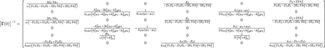
The convention follows the acronyms of Allard [All2009] , so see the detailed description there.

Use perforation at all plate-like infinite layers

In many applications plates or impervious screen layers are perforated. That means there is a fraction of motion given by the flow through the perforation of the plate. This is done by using the perforation keyword in the definition of the related infiniteLayers class.

We crate a perforate.

il_perforate   = iL.PerforatedLayer(0.005, 0.001, distance = 0.02)

Note that this doen’t need to be a PerforatedLayer this can also be a simple ResistiveLayer that just defines the transfer impedance of the layer.

The perforation is applied by the perforation keyword argument.

il_steel_5mm_perf = iL.PlateLayer(steel5mm,perforation = il_perforate)
il_steel_5mm_s_perf = iL.ImperviousScreenLayer(steel5mm,perforation = il_perforate)

The perforation does not change the parameters of the plate. Thus, the loss in stiffness and mass due to perforation must be considered by the user.

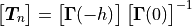
Coupling transfer matrices

When layers of different nature are interfacing specific matrices are required to define the conditions of these interfaces. In section 11.4.2 of [All2009] those interfaces are described in detail. Due to our nomenclature an interface occurs at the right node of layer $n$ with ${\rm NID}_{right} = 2n-1$ and the left node of layer $n+1$ with ${\rm NID}_{left} = 2(n+1)-1=2n+1$ . This can be for example the nodes 2 and 3.

Two layers of the same nature

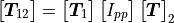
When two adjacent layers are connected and there is no poroelastic material involved, there layer matrices and degrees of freedom are organized in such a way that simple matrix multiplication gives the combined matrix. :

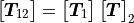
(11) $\begin{bmatrix} {\bm T}_{12} \end{bmatrix} = \begin{bmatrix} {\bm T}_1 \end{bmatrix} \begin{bmatrix} {\bm T} \end{bmatrix}_2$

In this case the final transfer matrix will have node 1 as output and node 4 as input. This makes this theory so practical when the nature of all layers is the same. When poroelastic materials are involved the porosity of each layer must be considered and an interface matrix becomes necessary. :

(12) $\begin{bmatrix} {\bm T}_{12} \end{bmatrix} = \begin{bmatrix} {\bm T}_1 \end{bmatrix} \begin{bmatrix} {I}_{pp} \end{bmatrix} \begin{bmatrix} {\bm T} \end{bmatrix}_2$

This matrix reads as:

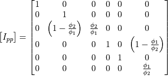
(13) $\begin{bmatrix} {I}_{pp} \end{bmatrix} = \begin{bmatrix} 1 & 0 & 0 & 0 & 0 & 0 \\ 0 & 1 & 0 & 0 & 0 & 0 \\ 0 & \left(1-\frac{\phi_2}{\phi_1}\right) & \frac{\phi_2}{\phi_1} & 0 & 0 & 0 \\ 0 & 0 & 0 & 1 & 0 & \left(1-\frac{\phi_1}{\phi_2}\right) \\ 0 & 0 & 0 & 0 & 1 & 0 \\ 0 & 0 & 0 & 0 & 0 & \frac{\phi_1}{\phi_2} \end{bmatrix}$

This matrix is defined by the I_porous_porous() function. This function generates a DynamicMatrix with the given node IDs as argument.

Two layers of the different nature

When such layers are interfacing the way how the different degrees of freedom are connected must be given. This is done be defining the conditions of for layer 1 and 2 and adjacent nodes 2 and 3 for example by:

(14) $\begin{bmatrix} {I}_{12} \end{bmatrix} \begin{Bmatrix} {\bm V}^{(1)}(2) \end{Bmatrix} + \begin{bmatrix} {J}_{12} \end{bmatrix} \begin{Bmatrix} {\bm V}^{(2)}(3) \end{Bmatrix} = \begin{Bmatrix} 0 \end{Bmatrix}$

The interface matrices are also given as a DynamicMatrix object. In this nomenclature the exc_dof of both matrices are clear, these are $\begin{Bmatrix}{\bm V}^{(1)}(2)\end{Bmatrix}$ and $\begin{Bmatrix}{\bm V}^{(2}(3)\end{Bmatrix}$ . Allard does not care about the res_dof because he simply lines up the the equations. As pyva uses the DynamicMatrix we have to define the res_dof that the entries will be considered in the final Allard matrix.

Solid-Fluid Interface

In order to explain the logics of the res_dof the solid-fluid interface is derived as example. We use the same layer and node IDs.

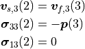
(15) ${\bm v}_{s,3}(2) &= {\bm v}_{f,3}(3) \\ {\bm \sigma}_{33}(2) &= -{\bm p}(3) \\ {\bm \sigma}_{13}(2) &= 0$

When writing this in matrix form it becomes clear that specific degrees of freedom determine the res_dof.

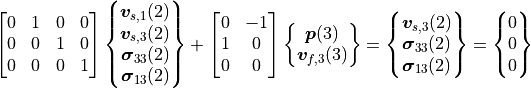
(16) $\begin{bmatrix} 0 & 1 & 0 & 0 \\ 0 & 0 & 1 & 0 \\ 0 & 0 & 0 & 1 \end{bmatrix} \begin{Bmatrix} {\bm v}_{s,1}(2) \\ {\bm v}_{s,3}(2) \\ {\bm \sigma}_{33}(2) \\ {\bm \sigma}_{13}(2) \end{Bmatrix} + \begin{bmatrix} 0 & -1 \\ 1 & 0 \\ 0 & 0 \end{bmatrix} \begin{Bmatrix} {\bm p}(3) \\ {\bm v}_{f,3}(3) \end{Bmatrix} = \begin{Bmatrix} {\bm v}_{s,3}(2) \\ {\bm \sigma}_{33}(2) \\ {\bm \sigma}_{13}(2) \end{Bmatrix} = \begin{Bmatrix} 0 \\ 0 \\ 0 \end{Bmatrix}$

Thus, a logical res_dof is $\begin{Bmatrix}{\bm v}_{s,3}(2) \\ {\bm \sigma}_{33}(2) \\ {\bm \sigma}_{13}(2)\end{Bmatrix}$ and ${\bm v}_{s,1}(2)$ is not part of it, because there is no condition defined.

When both layers are exchanged the matrices $[I]$ and $[J]$ are exchanged. But this means that the res_DOF is still linked to the ‘complicated’ layer of the connection, the solid. The res_dof is then similar, but connected to another node: $\begin{Bmatrix}{\bm v}_{s,3}(3) \\ {\bm \sigma}_{33}(3) \\ {\bm \sigma}_{13}(3)\end{Bmatrix}$

All this is taken into account in the methods hat generate the degrees of freedom of the Allard matrix, namely pyva.models.TMmodel.V0() and pyva.models.TMmodel.allard_matrix().