Properties package

The main purpose of the classes defined in the property package is to define the properties of systems and materials as far as populating the database.

Materials

The pyva.properties.materialClasses module contains classes for the description of materials. The classes falls into the acoustic or fluid category or the structure category.

Fluids

The pyva.properties.materialClasses.Fluid class deals with classical fluids or gases. In most vibroacoustic applications this is - to my surprise - air. Thus, air is the default setting in the constructor:

import pyva.properties.materialClasses as matC

air = matC.Fluid()

There are many parameters describing the fluid that are usually not that important unless they are required in porous material theory where viscosity and thermal properties become relevant.

print(air)
c0              : 343.0
rho0            : 1.23
nu0             : 1.4959349593495935e-05
eta             : 0.01
dynamic_visc    : 1.84e-05
Pr              : 0.71
kappa           : 1.4

There are many methods implemented to get the dynamic properties of fluids. In most cases there is a speciality in the implementation; most methods have a frequency keyword argument. This is implemented in such a way, to keep the door open for daughter classes with frequency dependent properties.

omega = np.geomspace(100,10000,5)
>>> air.c_freq(omega)
array([342.99142521+1.71495713j, 342.99142521+1.71495713j,
   342.99142521+1.71495713j, 342.99142521+1.71495713j,
   342.99142521+1.71495713j])

Note, that there is an imaginary component that comes from the eta = 0.01 in the default definition. When the real speed of sound is required, use

>>> air.c0
343.0

There are methods that determine acoustic properties at interfaces to other media. For, example the pyva.properties.materialClasses.Fluid.reflection_factor() and pyva.properties.materialClasses.Fluid.absorption() calculate the reflection_factor and absorption coefficient for plane interfaces to fluids with given impedance.

z1 = air.impedance()*1.5

reflection_factor = air.reflection_factor(omega, z1, theta = 0)
absorption_coefficent = air.absorption(omega, z1, theta = 0)

>>> absorption_coefficent
array([0.96, 0.96, 0.96, 0.96, 0.96])

Even though the perpendicular absorption is not perfect, the acoustic design goal for diffuse field absorbers should be 1.5 times the specific air impedance as it can be shown be the absorption_diffuse method

>>> absorption_diffuse    = air.absorption_diffuse(omega, z1)
>>> absorption_diffuse
array([0.9510412, 0.9510412, 0.9510412, 0.9510412, 0.9510412])

Other fluids can also be created by using the paramter list of the contructor:

water = matC.Fluid(c0=1500, rho0=1000,dynamic_viscosity=1.0087,eta = 0.)

Air properties under specific atmospheric conditions

In some applications the properties of air must be precisely known. For example in pressurise aircraft cabins that have lower static pressure conditions as on the ground or during tests of porous materials. In [Ras1997] the various papers defining all required properties are condensed in one numeric recipe. His equations are used to calculated the properties of air.

For this purpose there is the air() method that creates a Fluid object with the desired properties.

>>> air_10C_1013_20 = matC.Fluid.air(284.15,1.023,20) # (T in Kelvin, pressure in bar, humidity in %)
>>> print(air_10C_1013_20)
c0                : 338.1911712485711
rho0              : 1.253486363839927
nu0               : 1.4127054955709544e-05
eta               : 0
dynamic_visc      : 1.7708070748199177e-05
Cp                : 1007.2873957544533
heat_conductivity : 0.02448709290705875
Pr                : 0.7284293213363585
kappa             : 1.402275517294867

Note that eta is a global damping parameter that is not required when the viscosity of air is used. A frequency dependent eta can be defined from these properties.

Equivalent fluids

The equivalent fluids model is used for the simulation of very soft (limb) or very stiff (rigid) porous materials. This model is described in detail in [All2009] and briefly in [Pei2022]. The advantage of the equivalent fluid model is, that the state variables are the same as for fluids: pressure and velocity.

The number of parameters, models and model details is quite complex and study of related literature is strongly recommended. The following table summarises the parameters.

Symbol	Constructor argument	Description
$\rho_{bulk}$	rho_bulk	Density of absorber matrix and fluid
$\sigma$	flow_res	static air flow resistivity
$\Phi$	porosity	volume porosity
$\alpha_\infty$	tortuosity	tortuosity
$\Lambda$	length_visc	viscous characteristic length
$\Lambda'$	length_therm	thermal characteristic length
limp or rigid model	limp	switch

The equivalent fluid class is a daughter class of Fluid. Thus, the rest of the constructor parameters are the same as for fluids. For demonstration we create two equivalent fluids but with different limb switch settings

fibre_limp = matC.EquivalentFluid(porosity = 0.98, \
                               flow_res = 25000.,\
                               tortuosity = 1.02, \
                               length_visc = 90.e-6, \
                               length_therm = 180.e-6,\
                               rho_bulk = 31.176 , \
                               rho0 = 1.208, \
                               dynamic_viscosity = 1.81e-5 )

fibre_rigid = matC.EquivalentFluid(porosity = 0.98, \
                               flow_res = 25000., ...\
                               limb = False, \
                               ... dynamic_viscosity = 1.81e-5 )

Now, it will become obvious why some methods of the Fluid class are with frequency argument:

omega = np.geomspace(100,10000,100)

c_limp  = fibre_limp.c_freq(omega)
c_rigid = fibre_rigid.c_freq(omega)

rho_limp  = fibre_limp.rho_freq(omega)
rho_rigid = fibre_rigid.rho_freq(omega)

When the above results are plotted for real and imaginary part a strong frequency dependence can be seen. Both models differ very strongly at low frequencies but coincide for high frequencies.

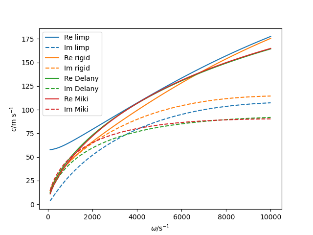
_images/equiv_sound_speed.png — Sound speed of equivalent fluid models.

_images/equiv_density.png — Density of equivalent fluid models.

Isotropic solid material

The elastodynamics of solids is modelled by complex matrices. For isotropic materials the situation is rather simple and the material is defined by mainly three parameters. The standard material is aluminium (from my aerospace background) but steel can be easily defined

alu   = matC.IsoMat()
steel = matC.IsoMat(E=2.1e11,rho0=7850, nu = 0.3)
print(alu)
E              : 71000000000.0
rho0           : 2700.0
nu             : 0.34
eta            : 0.01

The shear-modulus depends on the other constants and is therefore implemented as parameter method.

>>> alu.G
26492537313.432835

>>> steel.G
80769230769.23077

As damping is implemented all mechanical constants can be complex. This can be requested by specific methods

>>> alu.G_complex
(26492537313.432835+264925373.13432837j)

The bulk longitudinal and shear wave speeds are also implemented.

>>> steel.c_L
steel.c_L
6001.054841705961+30.004524114178846j)
>>> steel.c_S
(3207.6987395578053+16.038092755493444j)

When the damping component is not wanted, eta must be set to zero.

Geometrical properties

The geometry properties concerns properties that determine the dynamic behaviour by its shape. This can be an area of a tube or the thickness of a plate. As these properties are such simple they are given by a single parameter in the specific class, e.g. thickness of plates.

A very complex shape is the cross section of beams, thus the only geomtrical property defined here is the pyva.properties.geometricalPropertyClasses.CrossSection class.

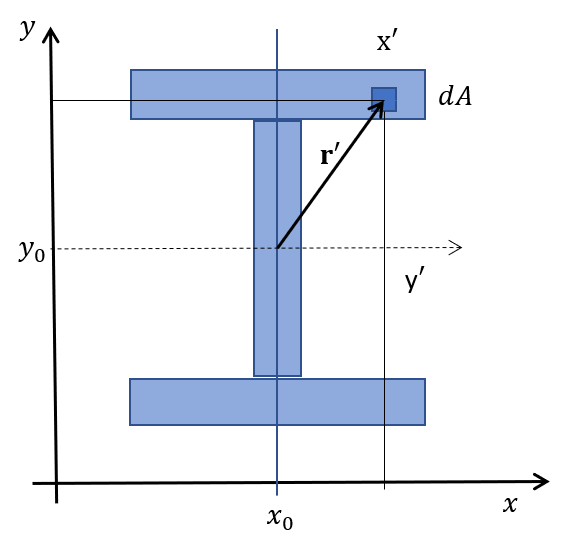
_images/cross_section.png — Beam cross section.

You can either enter the moments of area directly or use the constructor of a specific shape.

import pyva.properties.geometricalPropertyClasses as geoPC

# Beam constants
h    = 0.02
b    = 0.03

A    = h*b
Iz   = b**3*h/12
Iy   = b*h**3/12
Ixy  = 0.

beam_sec1 = geoPC.CrossSection(Ix, Iy, Ixy, A)
beam_sec2 = geoPC.RectBeam(Lx, Ly)

Both should have the same properties

print(beam_sec1)
print(beam_sec2)

leads to the following output

CrossSection:
Ix              : 4.499999999999999e-08
Iy              : 2.0000000000000004e-08
Ixy             : 0.0
area            : 0.0006

RectBeam:
Ix              : 4.499999999999999e-08
Iy              : 2.0000000000000004e-08
Ixy             : 0.0
area            : 0.0006
Lx              : 0.02
Ly              : 0.03

Structural properties

The structural properties are always a combination of geometric and material properties. They are part of the pyva.properties.structuralPropertyClasses module. It is imported via

import pyva.properties.structuralPropertyClasses as stPC

Beam properties

The attributes of the pyva.properties.structuralPropertyClasses.BeamProp class are the CrossSection and the material. As beam theory is usually restricted to isotropic material it is defined as that.

A beam prop is created with the above input by

beam_prop = stPC.BeamProp(beam_sec2,alu)

This means collecting a lot of parameters contained in the attribute cross_section and iso_mat:

print(beam_prop)
BeamProp:
cross_section:
RectBeam:
Ix              : 4.499999999999999e-08
Iy              : 2.0000000000000004e-08
Ixy             : 0.0
area            : 0.0006
Lx              : 0.02
Ly              : 0.03
iso_mat:
E              : 71000000000.0
rho0           : 2700.0
nu             : 0.34
eta            : 0.01

Important methods are related to bending, for example

>>> beam_prop.Bx
3194.9999999999995

>>> beam_prop.By
1420.0000000000002

Or point stiffness in specific directions that is required for coupling loss factor determination.

Plate properties

The basic model of a two-dimensional property is the thin Kirchhoff plate. With no complications as curvature, anisotropy or lay-ups. Even for a simple system the theory is so complex that many methods are implemented. The detailed description of all details is out of scope for this documentation. Please refer to [Pei2022] for the derivation.

In the future the idea it to include complications as curvature. This is an excellent task for others to enter.

The geometry parameter of plates is rather simple: It is just the thickness. Thus, the plate property is created with

alu   = matC.IsoMat()
alu4mm = stPC.PlateProp(0.004, alu)

Most of the implemented methods are required from other classes. For example the pyva.properties.structuralPropertyClasses.PlateProp.transfer_impedance() method that is used in the infinite layer applications of plates.

The junction classes required the semi infinite radiation stiffnesses from point in the infinite plate and along edges of the semi-infinite plate. There are three propagating wave types, longitudinal, shear and bending, the latter even as phase and group-wave speed. They are requested by

alu4mm.c_L()
alu4mm.c_S()
alu4mm.c_B_phase(omega)
alu4mm.c_B_group(omega)

The first two are usually not frequency dependent. The bending wave speed is frequency dependent which makes the frequency argument necessary and motivates the introduction of a group speed.

Poroelastic Materials

Poroelastic materials are a combination of porous materials (here implemented as EquivalentFluid) and elastic solids (implemented as IsoMat). As most parameters are from the EquivalentFluid) class, the IsoMat class is a subclass of this class.

The theory of poroelastic material was established in the late 50ties by M.A. Biot. This is the reason why many people talk about Biot materials instead of poroelastics. It is worth mentioning that the main achievements where made on new models ans descriptions of porous materials where made recently. Whereas the theory for the coupled dynamics was established by Biot much earlier. A comprising description of most models and theories are given by Allard ([All2009]).

Due to the fact that both models are implemented there are no additional parameters required for this type of material. For test and presentation purposes we use the material parameters from section 6.5.4 of [All2009].

E = 2*2200000.*(1+0.) # Calculate E from G in reference
ela_vac = matC.IsoMat(E,130., 0., 0.1) # Frame in vaccuum
poroela = matC.PoroElasticMat(ela_vac, \
                            flow_res = 40000., \
                            porosity = 0.94, \
                            tortuosity = 1.06, \
                            length_visc = 56.E-6, length_therm = 110.E-6)

There are numerous constants, coefficients and descriptions required to fully understand the underlying theory. So, if you are just using the poroelastic materials in specific layers without implementations a basic understanding of the main parameters is sufficient. With print the various parameters are summarized.

>>>print(poroela)
E              : 4400000.0
rho0           : 130.0
nu             : 0.0
eta            : 0.1
c0                : 343.0
rho0              : 1.23
nu0               : 1.4959349593495935e-05
eta               : 0.0
dynamic_visc      : 1.84e-05
Cp                : 1005.1
heat_conductivity : 0.0257673
Pr                : 0.717725178811905
kappa             : 1.4
flow_res          : 40000.0
porosity          : 0.94
tortuosity        : 1.06
rho_bulk          : 131.1562
lentgh_visc       : 5.6e-05
lentgh_therm      : 0.00011

If you think about your own applications using the poroelastic models a deep study of [All2009] is not only recommended.

The main effect of the coupled formulation, is that there are two compressional waves and one shear wave. The squared wavenumbers and the ration of their amplitudes between air and solid motion are calculated with wavenumbers().

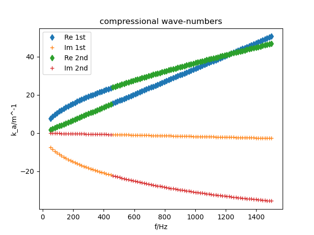
_images/biot_compressional_wavenumbers.png — The compressional wavenumbers of a poroelastic material.

In figure The compressional wavenumbers of a poroelastic material. the wavenumber of the two compressional waves are shown. Note, that the curves are switching. This is due to the numerical implementation of the square root. This does not have an impact on the implementation because both numbers can be interchanged.

The same effect occurs when the characteristic impedances are calculated with impedances().

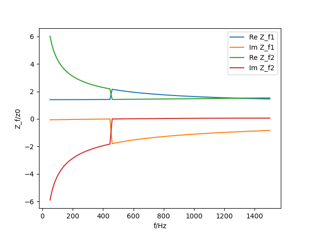
_images/biot_fluid_impedances.png — The characteristic fluid impedances of a poroelastic material.

_images/biot_structure_impedances.png — The characteristic structure impedances of a poroelastic material.

All curves are in perfect agreement with Allards results.