Systems package

The systems sub-package pyva.systems provide several modules for the [All2009] of various dynamic systems. At first all classes have attributes to describe each system in an appropriate way. This includes the topology, the properties and the materials that are used to build up the system.

If possible the SEA- and deterministic descriptions for each subsystem is provided. That means that each class have methods that generate a local SEA_model, VAmodel, FEM or TMmodel.

The systems subpackage is organised by the topology (one-, two- or three-dimensional) and nature (structure or acoustic) of the systems. Zero dimensionsional systems are considered in the lumped systems module pyva.systems.lumpedSystems and the SEA_system module exclusively contains the abstract base class for all possible SEA systems.

The foundation of the system modules is given in chapters 1,4,5 and 6 of [Pei2022].

_images/systems_overview.png — Topology logics of structure and acoustic systems

In addition there are system like objects. They are special in that sense that they are infinite in at least one dimension. But even a half space has a response to an excitation and can therefore be considered as a system. This concerns all kind of sources and radiators in the fluid domain pyva.systems.acousticRadiators and the infinite layers that are mandatory for the noise control treatment [All2009] pyva.systems.infiniteLayers. There is lumpedSystems module that includes a harmonic oscillator class mainly aimed at documentation for the book creation of [Pei2022].

_images/special_systems_overview.png — Modules for special systems

SEA_system

This class is the abstract base class for all SEA systems. All daughter classes are obliged to implement specific methods, that are required for SEA [All2009]. Those methods represent the functions or parameters required for SEA simulation.

One important detail of SEA system classes is that an ID attribute is mandatory. From this ID and the physical properties, the wave degree of freedom is created. For example the degree of freedom of a cavity SEA system of ID=4 is DOF(4,0,typestr=’pressure’). The DOF of SEA systems is similar to the DOF of nodes in deterministic models but here related to reverberant wave fields.

Acoustic Systems

Systems that are constituted by fluid volumes are considered as acoustic systems. In both classes the fluid is described by the Fluid class pyva.properties.materials.Fluid or subclasses.

The topology is restricted to one- and three dimensional systems because two-dimensional systems are either rarely used in real applications or can be modelled by a infinite fluid layer pyva.systems.infiniteLayers.AcousticLayer

One dimensional acoustic systems

One dimensional acoustic systems are pipes and tubes with cross section much smaller than occurring wavelengths. Due to the fact that such systems are hardly random, this class is not an extension of the SEA_system class.

In general the pyva.systems.acoustic1Dsystems module deals with acoustic networks of pipes, perforated layer, lumped elements of specific set-ups as the HelmholtzResonator or the QuarterWaveResonator. The all have in common that they can be described by a transfer- or mobility-matrix with the volume flow and pressure as degrees of freedom. Depending on the representation the sign convention is different. For the transmatrix therory the pressure (or force) is considered as an internal pressure that has negative sign compare to the finite element presenation. This is required to allow for the practical series matrix multiplication. See [Pei2022] for details.

These one-dimensional system can be combined to create acoustic networks. This is described in more detail in Acoustic network.

Acoustic tubes

_images/acoustic_tube.png — Acoustic tube or pipe set-up

Acoustic tube set-up, parameters and degree of freedom. When tubes are used in acoustic networks it is helpful to use the volume flow instead of velocity, this is more appropriate for changing cross sections.

A simple tube can be generated by the following code.

>>> air = matC.Fluid()
>>> L = 1.
>>> S = 0.01

>>> tube = ac1Dsys.AcousticTube(L,air,S)

>>> tube
AcousticTube(1.0,fluid=Fluid(c0=343.0,rho0=1.23,eta=0.01),S=0.01)

From this set-up elements can be created by using the pyva.systems.acoustic1Dsystems.AcousticTube.acoustic_FE() method. For later use in the FE context the node ID must be selected:

>>> omega = np.linspace(100.,200.,11)
>>> tube_elem = tube.acoustic_FE(omega,ID =[1,2])

The outcome is a VAmodel representation of this tube in the desired frequency range

>>> tube_elem
LinearMatrix of size (2, 2, 11), sym: 1
DataAxis of 11 samples and type angular frequency in hertz
resdof: DOF object with ID [1 2], DOF [1 1] of type [DOFtype(typestr='volume flow')]
excdof: DOF object with ID [1 2], DOF [0 0] of type [DOFtype(typestr='pressure')]

Lumped acoustic systems

Lumped acoustic systems are a kind of obstacle that are positioned in the fluid flow and that can be represented by one transfer impedance. Thus, the transfer impedance is the key attribute for the description of the lumped behaviour. For maximum flexibility the transfer impedance must be given as a function of omega, but can also be a constant. This class is basically a base class for the implementation of acoustic network models of a physical set-up like mass layers, perforates and membranes.

_images/lumped_1D.png — Transfer impedance representation of lumped elements

Mass, stiffness (and damping) layer

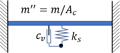
_images/mass_stiffness_1D.png — Lumped element model of condensed mass, stiffness and damping

The most simple lumped system is a layer with mass, stiffness and damping properties. The acoustic transfer impedance of such systems is:

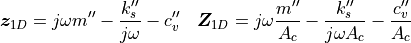
(1) $\bm{z}_{1D} = j\omega m''-\frac{k''_s}{j\omega}- c''_v \quad \bm{Z}_{1D}= j\omega \frac{m''}{A_c} -\frac{k''_s}{j\omega A_c} -\frac{c''_v}{A_c}$

The double prime denotes per area, e.g. $m''=m/A_c$ . A mass, stiffness layer object is created by:

>>> mass_stiffnes_layer = ac1Dsys.MassStiffness(0.001, 2.)

Note, that the class attributes are the total mass, stiffness etc. and are converted into area specific values by division with the cross section area. In addition to the viscous damping the damping can also be defined as damping loss $\eta$ that is considered as imaginary part of the stiffness $\bm{k}_s=k_s(1+j\eta)$ .

Membrane

A membrane is a flat surface under tension, without bending stiffness like an ideal drumhead. The membrane dynamics is determined by the shape, mass and weight of the membrane. The related model is described in [Pei2022].

The membrane mass is defined via the density of the material and the thickness.

>>> rubber = matC.Fluid(1500,1.1)
>>> T = 200    # tension
>>> h = 0.001  # thickness
>>> my_mem = ac1Dsys.membrane(rubber,h,T,S)

The output of the membrane is given as MassStiffness object:

>>> my_mem
MassStiffness:
m              : 1.46667e-05
k_s            : 1600
c_v            : 0
eta            : 0
area           : 0.01

Note that the efficient mass higher than the corresponding mambrane mass according the the membrane model [Pei2022].

Perforated layer

Perforated layer constitute one of the most important mean in noise control. This results from the fact that by choosing a specific perforation the transfer impedance can be designed to appropriate values.

See the following sketch for the perforate definition.

_images/perforate.png — Definition of perforate

The perforate model simulates the flow through the small channels in the perforate. The flow in the small tubes generate a mass correction on both sides of the perforate und damping because of viscous flow. According to Peiffer [Pei2022] this leads to a transfer impedance due to the given model.

The porosity is either calculated from distance, radius and pattern or directly given.

A typical perforate can be generated with:

>>> thickness = 0.002
>>> holeR     = 0.0001
>>> dist      = 0.01

>>> perf = ac1Dsys.PerforatedLayer(thickness,holeR,distance = dist)

The porosity of the perforate can be requested.

>>> perf.porosity
0.0003141592653589793

The important quantity is the transfer impedance can be visualised using the plot method

>>> omega = 2*np.pi*np.linspace(1.,1000.)
>>> perf.plot(omega,res='real')

Leading to the following result

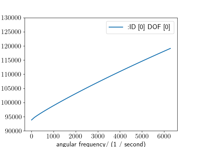
_images/perforate_resistance.png — Perforate resistivity

Helmholtz resonator

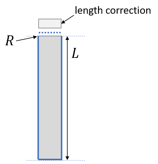
A Helmholtz resonator is in contrast to the above two-port examples a one port system. In the transfer impedance description this means a state vector with specific ratio of pressure and (volume)velocity. In the VAmodel description this corresponds to a nodal mobility value. The geometry of the Helmholtz resonator is depicted in the following.

_images/helmholtz.png — Sketch of Helmholtz resonator

The main constructor parameters follow from figure Sketch of Helmholtz resonator. In addition the transfer impedance on the neck cover can be given and the end-correction length that defaults to 1.7 times the radius for both sides can be set.

We create two resonators, one with an one without a perforate with specific parameters

>>> thickness = 0.0002
>>> holeR     = 0.0001
>>> porosity  = 0.0072

The Helmholtz parameters are as follows:

>>> V         = 0.000001
>>> L         = 0.005
>>> R         = 0.002
>>> Ac        = np.pi*R**2

Perforate and resonators are created using the related constructors. Note that the end correction is reduced to the half because the perforate doesn’t require an end correction on top.

>>> perf_HR    = ac1Dsys.PerforatedLayer(thickness,holeR,Ac,porosity = dist)
>>> myResPure  = ac1Dsys.HelmholtzResonator(V,L,R,air)
>>> myResPerf  = ac1Dsys.HelmholtzResonator(V,L,R,air,0.85,end_impedance=perf_HR.radiation_impedance)

With a new appropriate frequency range, the results can be calculated using the acoustic_impedance method.

>>> omega = 2*np.pi*np.linspace(100.,5000.,200)
>>> Za_pure = myResPure.radiation_impedance(omega)
>>> Za_perf = myResPerf.radiation_impedance(omega)

and plotted with matplotlib.

>>> plt.figure()
>>> plt.plot(omega,np.real(Za_pure),label = 'Re pure')
>>> plt.plot(omega,np.imag(Za_pure),label = 'Im pure')
>>> plt.plot(omega,np.real(Za_perf),label = 'Re perf')
>>> plt.plot(omega,np.imag(Za_perf),label = 'Im perf')
>>> plt.xscale('log')
>>> plt.legend(loc=4)
>>> plt.show()

_images/HR_acoustic_impedance.png — Acoustic impedance of both Helmholtz resonator

Quarter wave resonator

When wavelengths are getting smaller the simple model of the air volume acting as spring is not correct. When the volume fulfils the assumption of one-dimensional systems it can be modelled as tube. This is implemented in this class.

The parameters of the constructor are similar except the skipped volume parameter. The resonator is generated via the following code snipped:

>>> quarter_perf  = ac1Dsys.QuarterWaveResonator(4*L,R,air,0,end_impedance=perf.radiation_impedance)
>>> Za_perf = quarter_perf.radiation_impedance(omega)

Using matplotlib

plt.figure()
plt.plot(omega,np.real(Za_perf), label = 'Re perf')
plt.plot(omega,np.imag(Za_perf), label = 'Im perf')
plt.xscale('log')
plt.legend(loc=4)
plt.show()

leads to the following result:

_images/QWR_acoustic_impedance.png — Acoustic impedance of QWR resonator

Three dimensional acoustic systems

Three dimensional acoustic systems are cavities or rooms (if very large). The base class is pyva.systems.acoustic3Dsystems.Acoustic3DSystem that model the cavity based on global properties as volume, surface and perimeter and the included fluid, further detailed by absorption quantities. This model is random and simulates the cavity as a reverberant field.

The base class is extended by the pyva.systems.acoustic3Dsystems.RectangularRoom class that provide in addition deterministic methods as modal analysis and frequency response.

We use the rectangular room class to present both, the deterministic and random capabilities.

>>> import numpy as np
>>> import matplotlib.pyplot as plt

>>> import pyva.systems.acoustic3Dsystems as ac3Dsys
>>> import pyva.properties.materialClasses as matC

>>> # Define default fluid
>>> air = matC.Fluid()

>>> # Cavity Parameters
>>> Lx = 6.
>>> Ly = 4.
>>> Lz = 3.

Details can be derived from the string representation

>>> room = ac3Dsys.RectangularRoom(1, Lx, Ly, Lz, air)
>>> print(room)
SEA cavity system with ID:1
volume          : 72.0
surface         : 108.0
perimeter       : 52.0
fluid:
--------
c0              : 343.0
rho0            : 1.23
nu0             : 1.4959349593495935e-05
eta             : 0.01
dynamic_visc    : 1.84e-05
Pr              : 0.71
kappa           : 1.4
damping_type    : ['eta']

Note that volume, surface and perimeter are automatically created. The damping_type attribute defines which damping is taken. The default is the the natural damping of the fluid.

As mentioned the deterministic nature on the rectangular room can be used to check the approximative methods for modal density estimation.

>>> omega = np.geomspace(100,10000,num=64)

>>> mod_dens              = room.modal_density(omega)
>>> mod_dens_precise,om_c = room.modal_density_precise(omega)

Note, that the precise method provides a new omega axis om_c, because the frequencies are interpreted as interval limits. The plotted results show that once the cavity can be considered as random, the estimation is not too bad.

_images/room_modal_density.png — Estimated and counted modal density

Structure Systems

There are no three-dimensional structure systems because they usually don’t exist in technical set-ups.

One-dimensional structural systems

Typical one-dimensional systems are beams, bars or rods. Here, a beam class is implemented and mainly modelling the bending motion in one direction. As described in [Pei2022] the 1D systems are random in very few cases. Thus, the implemented methods are deterministic methods to calculate the modal frequency response.

In further implementations the beams can be considered as a deterministic component of line junction as shown in [Lan1990]. For use in a script four modules of pyva must be imported:

import pyva.systems.structure1Dsystems as st1Dsys
import pyva.properties.materialClasses as matC
import pyva.properties.geometricalPropertyClasses as geoPC
import pyva.properties.structuralPropertyClasses as stPC

A beam instance is created with a length and property parameter that describes the beam.

alu = matC.IsoMat() # Alu is default

# Beam constants
# First example for oscillator
h    = 0.0005
b    = 0.0005
L    = 2

# Cross section
beam_section = geoPC.RectBeam(h, b)
# Beam property
beam_prop    = stPC.BeamProp(beam_section,alu)

beam = st1Dsys.beam(L,beam_prop)
print(beam)

with the output:

beam:
L               : 2
beam_prop:
BeamProp:
cross_section:
RectBeam:
Ix              : 5.2083e-15
Iy              : 5.2083e-15
Ixy             : 0.0
area            : 2.5e-07
Lx              : 0.0005
Ly              : 0.0005
iso_mat:
E              : 71000000000.0
rho0           : 2700.0
nu             : 0.34
eta            : 0.01

Two-dimensional structural systems

Two dimensional structure systems are flat plates and cylindrically or doubly curved shells. The single current implementation is the (thin) and flat Kirchhoff plate.

The creation of two-dimensional subsystems require the following imports:

import pyva.systems.structure2Dsystems as st2Dsys
import pyva.properties.materialClasses as matC
import pyva.properties.structuralPropertyClasses as stPC

Generic two-dimensional plate system

The pyva.systems.structure2Dsystems.Structure2DSystem is the generic, more SEA like version that has area and surface as parameter. A plate subsystem is create for example by

# Define the properties
alu = matC.IsoMat() # Alu is default

# Plate constants
h    = 0.02
Lx   = 2
Ly   = 3
area = Lx*Ly
perimeter = 2*(Lx+Ly)

# Plate property
plate_prop    = stPC.PlateProp(h,alu)

plate = st2Dsys.Structure2DSystem(1, area, plate_prop, perimeter = perimeter)

Note, that this is a subclass of SEA_system and that the constructor requires an ID argument. In general the generic Sructure2DSystem description is sufficient for random modelling of plates except the radiation efficiency that is estimated by the assumption that a rectangular plate with same area $A$ and perimeter $P$ has similar radiation efficiency.

$A &= L_x L_y \\ P &= 2(L_x + L_y)$

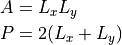
Therefore, the Structure2DSystem hat Lx- and Ly-methods to provide these edge lengths.

>>> plate.Lx
3.0

>>> plate.Ly
2.0

Lx and Ly are exchanged compared to the above code snipped, because Lx is always the larger dimension. When P=0 the plate is assumed to be square.

An important (acoustic) property is the radiation efficiency. This can be calculated using Leppingtons theory [Lep1982] or the more simple ISO EN 12354-1 method.

omega = np.geomspace(100,10000)
freq  = omega/2/np.pi

rad_eff = plate.radiation_efficiency(omega)
rad_eff_simple = plate.radiation_efficiency_simple(omega)

Resulting in the following graphs:

_images/plate_radiation_efficiency.png — Radiation efficiency calculated by different methods

The pyva.systems.structure2Dsystems.Structure2DSystem class provides many further methods that are required to allow the use of such systems in SEA models. This comprises the edge radiation stiffnesses that are part of the property classes because the dynamics of the semi-finite radiation stiffness depends only on plate properties and not on the geometry of the plate.

The transmission loss of plates is calculated in SEA using the non-resonant paths (that represents the mass law) and the resonant path that uses the radiation efficiency for the determination of the coupling loss factor. However, when noise control treatment is applied to the plate the impact of the treatment to the transmission is calculated using the insertion loss of the trimmed to the untrimmed configuration. In this case the wavenumber transmission formulas can be used in contrast to pure plates where the infinite plate theory fails at coincidence.

Thus, for the trim and mass law tasks this class provides methods that create an instance of the pyva.models.TMmodel class.

The plate system can be covered with noise control material, so called trim. The trim must be given as transfer matrix model, as described in the Infinite Layers section.

The Rectangular Plate

The pyva.systems.structure2Dsystems.RectangularPlate class is extension of pyva.systems.structure2Dsystems.Structure2DSystem with a more specific geometry. Due to this and the fact that analytical solutions are available. This class contains additional deterministic methods for the modal response. A RectangularPlate instance is generated by:

rec_plate = st2Dsys.RectangularPlate(2, Lx,Ly, prop=plate_prop)

The pyva.systems.structure2Dsystems.RectangularPlate.w_mode() method provides the mode shape of double index n=(nx,ny). This is used in pyva.systems.structure2Dsystems.RectangularPlate.w_modal_force() to calculate the frequency response of normal excitation.

First, the highest mode index for required frequency must be found. This can be done by pyva.systems.structure2Dsystems.RectangularPlate.get_modes_index() that calculates a sorted mode index an provides the highest index:

>>> _,Ns = rec_plate.get_modes_index(omega[-1])
>>> N_max = Ns[-1]
>>> N_max
array([18, 33])

For example the displacement amplitude at the excitation point is calculated as follows uswing the same coordinates for excitation and response:

x0 = 0.71
y0 = 1.22
w0 = rec_plate.w_modal_force(omega, N_max, 1., x0, y0, x0, y0)

For demonstration purpose the infinite plate displacement is also calculated.

   w0_inf = rec_plate.prop.w_inf(omega,0., 1.)

.. _fig-plate_radiation_efficiency:

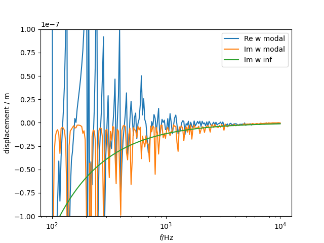
_images/plate_point_displacement.png — Point displacement due to normal unit force.

Note, that the point displacement of infinite plate is imaginary for real excitation amplitude. An interesting feature of the rectangular plate class is possibility to calculate the transmission loss using hybrid methods and a discrete or modal representation.

First, the discrete mathods require a pyva.geometry.meshClasses.RegMesh2D instance. This is created using the pyva.systems.structure2Dsystems.RectangularPlate.get_mesh() method. We create a thicker and smaller plate to keep calculation time reasonable:

Lx = 0.8
Ly = 0.5
h  = 0.004

plate_prop  = stPC.PlateProp(h,alu)
rec_plate   = st2Dsys.RectangularPlate(3, Lx,Ly, prop=plate_prop, eta = 0.05)

A :class_`~pyva.systems.acousticRadiators.HalfSpace` of air must be created

half_air = aR.HalfSpace()

First, we calculate the modal transmission coefficient using the modal hybrid method:

tau_modal = rec_plate.modal_transmission_coefficient_discrete(omega,(half_air,),)

See chapter 11 of [Pei2022] for details. In addition (but mainly for demonstration purposes) the transmission coefficient can be calculated using the discrete radiation stiffness and the point force transfer functions of flat plates. Thus, the radiating area is assumed to be finite but the plate is infinite:

tau_inf   = rec_plate.transmission_coefficient_discrete(omega, (half_air,))

Applying both methods provide the following transmission loss results.

_images/plate_transmission_discrete.png — Transmission loss from two different discrete methods.

A very simple but useful method is pyva.systems.structure2Dsystems.RectangularPlate.normal_modes(). This method is used internally in the modal transmission loss method and generate numerical mode shapes by simple mapping of the analytical solution to a mesh:

mode_shapes,mesh = rec_plate.normal_modes(5000.)

The result is a ShapeSignal those mode shapes can be plotted by:

mode_shapes.plot3d(4,1)

_images/plate_mode.png — First mode of plate.

Special systems

The special systems have a somehow infinite character. The have an input and output relation but are not closed as the systems described above.

Acoustic radiators

The acoustic radiations module contains classes for calculating the radiation of sound into the free or semi-finite half space. Beside some monopole or breathing sphere classes for demonstration purpose (or later point junctions), the most important classes are the Halfpace and the CircularPiston Class.

The pyva.systems.acousticRadiators.HalfSpace deals with methods for acoustic radiation into the semi-infinite half space and is therefore a key element for the junction formulation of the Area Junction.

The constructor has two main parameters: the fluid and a treatment argument:

import pyva.properties.materialClasses as matC
import pyva.systems.acousticRadiators as acR

air   = matC.Fluid()

HS = acR.HalfSpace(air)

omega = np.geomspace(100,10000,5)
omega0 = 1000.

The main category of methods deals with the radiation sound from vibrating surface for different degrees of freedom. The classical and simple radiation stiffness is in the wavenumber domain

kx_max = air.wavenumber(omega0)
kx = np.linspace(0,2*kx_max,200)

D_wavenumber = HS.radiation_stiffness_wavenumber(omega0, kx)

Plotting this pure imaginary stiffness for air without damping shows the typical shape radiation stiffness until k_x has reached the maximum wavenumber in air with singularity and zero stiffness for wavenumber k_x larger that in air (or below coincidence).

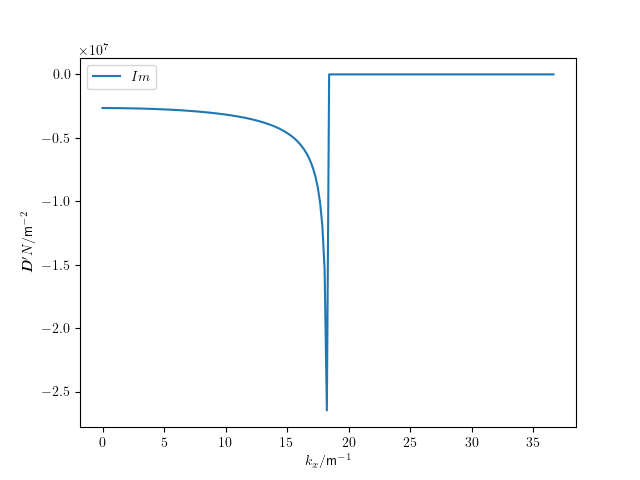
_images/half_space_stiffness_wavenumber.png — Stiffness of half space over wavenumber at 1000Hz.

An alternative way for the calculation of the radiation stiffness is the Leppington method [Lep1982] that considers the finite dimension of the radiator (already presented in the context of plate systems Generic two-dimensional plate system). Leppington did not calculate the radiation stiffness but the radiation efficiency that ca be used to derive the radiation stiffness. We define rectangular plate dimensions and call the related method

# Radiator dimensions
Lx = 0.8
Ly = 0.5

# Number of half sine wave on rectangle
nx = 10
ny = 3
# Corresponding wavenumber
kx = np.pi*nx/Lx
ky = np.pi*ny/Ly

sigma_LEP = HS.radiation_efficiency_leppington(omega,kx,ky,Lx,Ly,simple_muGT1=True)

A further option to get the radiation efficiency is to use mesh base methods that are presented later in more detail. Together with a shape function and the Reg2Dshape method the discrete shape function is generated.

Nx = 40
Ny = 25

shapefun = lambda x,y: np.sin(kx*x/Lx)*np.sin(ky*y/Ly)

This is not to be confused with the mode shaped of the rectangular plate that is only valid for one specific modal frequency. Here, the shape does not change over frequency

my_shape  = meshC.RegShape2D(0,0,Lx,Ly,Nx,Ny,shape = shapefun)
sig_sigma = HS.shape_radiation_efficiency(omega,my_shape,'wavelet')

When both results are plotted we see that both solutions coincide quite well

_images/half_space_sigma.png — Radiation efficient of sinusoidal shape.

There are many mesh based methods for the determination of the half space radiation stiffness of a regular mesh. The base of these methods is the local stiffness function. The wave motion of one element with displacement u creates a pressure at another element according to the Rayleigh integral. There are two versions implemented:

The wavelet method [Lan2007]
The piston method [Pei2022]

_images/half_space_mesh.png — Mesh and radiator and receiver.

The pressure at the receiving element leads to a force on the element and hence the stiffness can be easily calculated

(2) $\bm{D}_{ji} \bm{u}_i = \bm{F}_j$

For the calculation only the distance from node i to j is important. For this task we need a distance and the mesh element area

dist = 0.4
dA = my_shape.dA

The piston radiation stiffness according to Peiffer [Pei2022] is found with

D12piston = HS.radiation_stiffness_piston(omega, dist, dA, dA )
D11piston = HS.radiation_stiffness_piston(omega, 0., dA, dA )

The wavelet method [Lan2007] requires the mesh wavenumber ks

ks = my_shape.ks

D12wavelet = HS.radiation_stiffness_wavelet(omega, dist, ks)
D11wavelet = HS.radiation_stiffness_wavelet(omega, 0., ks)

In the following figure the difference between both methods is shown

_images/half_space_D12.png — Radiation stiffness for elements with distance.

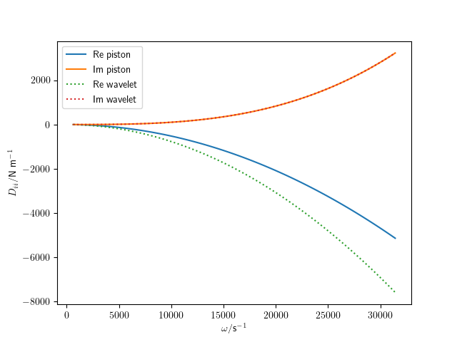
_images/half_space_D11.png — Self radiation stiffness.

The imaginary part of both stiffnesses are very similar. Only the reactive and real part of both methods differs. As Langleys method is supposed to be more precise, it is recommended if inertia effects are important.

Both methods are organised such as one parameter of dist or omega must be scalar. The return value has the dimension of the ndarray input, in this example the omega parameter.

There is a method to create to appropriate mesh from the maximum wavelength and dimensions

mesh     = HS.get_mesh(omega[-1], Lx, Ly; N=4)
>>> mesh
RegMesh2D(0.0,0.0,0.8,0.5,48,31,doftype =DOFtype(typestr='general'))

The radiation stiffness matrix of a mesh is calculated with

D_1000 = HS.radiation_stiffness_mesh_single([omega0], mesh,method = 'wavelet')

>>> D_1000
LinearMatrix of size (1488, 1488, 1), sym: 1
First matrix up to index 5 at iz = 0 ...

It is not recommended to calculate the stiffness matrix for several frequency lines in one shot, because the three dimensional array can become very large even though symmetry is used. The calculation may be surprisingly fast for an interpreter like Python, but the trick is that there are several equal distances in a regular mesh and the radiation stiffness is calculated once for one distance and then used for all node combination with equal distance.

The circular piston is useful for radiation of loudspeakers or tube end radiation into the half space. A piston instance is created by

radius = 0.3
my_piston = acR.CircularPiston(radius,fluid=air)

The radiation impedance of such a system is calculated with

rad_impedance = my_piston.acousticImpedance(omega)

Leading to the following figure.

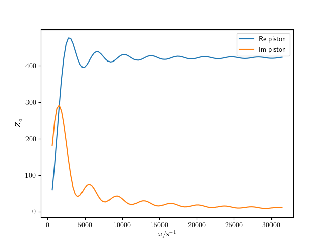
_images/piston_acoustic_impedance.png — Acoustic radiation impedance of circular piston.

For use in acoustic networks there is an pyva.systems.acousticRadiators.CircularPiston.acoustic_FE() method that calculates the nodal FE function for half space piston end conditions.