Acoustic network

This section describe the application of one-dimensional systems in an acoustic network. If the network is a sequential connection of systems the transfer matrix model can be used. Here, we present the capabilities of the pyva.models.VAmodel that provide much more flexibility because with this class branches and arbitrary network shapes can be easily created.

The required imports for the examples are:

import pyva.data.dof as dof
import pyva.systems.acoustic1Dsystems as ac1D
import pyva.systems.acousticRadiators as acR

import pyva.properties.materialClasses as matC
import pyva.data.matrixClasses as mC
import pyva.models as mds
import pyva.loads.loadCase as lC

Expansion chamber

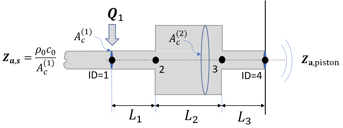
A classical device for noise control in exhaust or ventilation systems is the expansion chamber. This is a pipe section with a middle section of larger diameter and specific length as shown in the following figure.

Expansion chamber set-up.

We suppose a free field at the input and start with the materials and parameter section:

# Define frequency axis
xdata  = mC.DataAxis(2*np.pi*np.arange(10,1000,5),typestr='angular frequency')

# Tube parameter
R1 = 0.05
R2 = R1*np.sqrt(10)
R3 = 0.05

A1 = np.pi*R1**2
A2 = np.pi*R2**2
A3 = np.pi*R3**2

L1 = 0.2
L2 = 0.3
L3 = 0.2

# The fluid
air   = matC.Fluid(eta=0.01)

First, we create the specific AcousticTubes

tube1 = ac1D.AcousticTube(L1,air,A1)
tube2 = ac1D.AcousticTube(L2,air,A2)
tube3 = ac1D.AcousticTube(L3,air,A3)

For the comparison to a reference system a similar tube of full length and small cross section is created

tube_ref = ac1D.AcousticTube(L1+L2+L3,air,A1)

We suppose a flanged free half space, so the system we need for radiation is the pyva.systems.acousticRadiators.CircularPiston

end4  = acR.CircularPiston(R3,air)

For all these systems we use the acoustic_FE method

# Create finite elements
elem1 = tube1.acoustic_FE(xdata,ID=[1,2])
elem2 = tube2.acoustic_FE(xdata,ID=[2,3])
elem3 = tube3.acoustic_FE(xdata,ID=[3,4])
rad4  =  end4.acoustic_FE(xdata,ID=[4])
rad4free  =  air.acoustic_FE(xdata,A3,ID=[4])
entry4free  =  air.acoustic_FE(xdata,A1,ID=[1])
elem_ref = tube_ref.acoustic_FE(xdata,ID=[1,4])

Please, note the use of each required ID or ID pair in the element creation. In order to create the models a mesh must be defined that holds the nodal information

# Define required DOFtype
Qdof = dof.DOFtype(typestr=('volume flow'))
Pdof = dof.DOFtype(typestr=('pressure'))
# Nodes
NIDs   = [1,2,3,4]
# Response and excitation DOFs
excdof = dof.DOF(NIDs,[0],Pdof,repetition = True )
resdof = dof.DOF(NIDs,[1],Qdof,repetition = True )

With this preparation the empty models can be initialized

tube_network     = mds.VAmodel(None,xdata, excdof, resdof, sym=1, dtype=complex)
tube_ref_network = mds.VAmodel(None,xdata, excdof[0:4:3], resdof[0:4:3], sym=1, dtype=complex)

Due to the fact that each element comes with defined IDs the elements are simply added to the models:

# Expension chamber
tube_network += elem1
tube_network += elem2
tube_network += elem3
tube_network += rad4
tube_network += entry4free

# Same for reference
tube_ref_network += elem_ref
tube_ref_network += rad4
tube_ref_network += entry4free

Next step is the creation of a load

volume_source = lC.Load(xdata, 0.001*np.ones(len(xdata)), dof.DOF([1],[1],Qdof), name = 'VolumeFlow')
tube_network.add_load({1:volume_source})
tube_ref_network.add_load({1:volume_source})

and solving with loadresponse=True

tube_network.solve(loadresponse=True)
tube_ref_network.solve(loadresponse=True)

With this option the net volume flow is calculated. Due to the entry condition the actual volume flow that enters the system is different to the volume flow defined by the load. When we check the content of the model we can identify loads and results

>>> tube_network
LinearMatrix of size (4, 4, 253), sym: 1
DataAxis of 253 samples and type angular frequency in 1 / second
resdof: DOF object with ID [1 2 3 4], DOF [1 1 1 1] of type [DOFtype(typestr='volume flow')]
excdof: DOF object with ID [1 2 3 4], DOF [0 0 0 0] of type [DOFtype(typestr='pressure')]
Load with ID=1 Signal of 253 samples and 4 DOFs
Results with ID=1 Signal of 253 samples and 4 DOFs

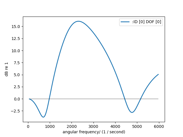
The results can be plotted with the usual methods for signals. The power() method calculates the power flow through the nodes:

pow_in  = tube_network.power(1,1)
pow_in.plot(10)
pow_out = tube_network.power(1,4,boundary = rad4) #free
pow_out.plot(10,cs='r')

leading to the following plot

Expansion chamber in- and output power of expansion chamber

The same can be done for the reference:

pow_in  = tube_ref_network.power(1,1)
pow_ref  = tube_ref_network.power(1,4,boundary = rad4)

leading to the following plot.

Expansion chamber in- and output power of expansion chamber

The insertion loss is determined using the transfer method of the Signal class

IL = pow_out.transfer(pow_ref,IDs=[4,4])
IL.plot(13,res = 'dB')

Leading to the following figure

Expansion chamber insertion loss

Helmholtz resonator in pipe

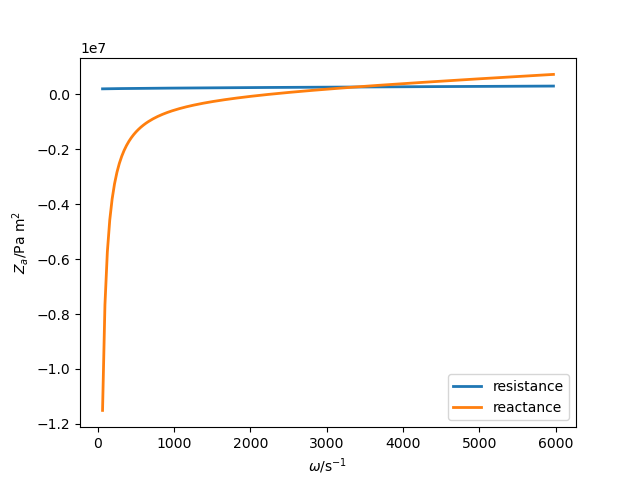
A further means of noise reduction is a Helmholtz resonator located in the pipe. The resonator is tuned at a certain frequency and works well for tonal noise issues for example in hydraulic pipes or for air intakes.

Helmholtz resonator as T-joint example

We define the frequency data and the dimensions of the set-up by the following variables:

# Define frequency axis
deltaF = 5
f0     = 10
f1     = 6000/2/np.pi
xdata  = mC.DataAxis(2*np.pi*np.arange(f0,f1,deltaF),typestr='angular frequency')

# Tube parameter
R1 = 0.01
A1 = np.pi*R1**2

L1 = 0.20
L3 = 0.20

# The fluid
air   = matC.Fluid(eta=0.0001)

# Perforate parameter
thickness = 0.0002
holeR     = 0.0001
porosity  = 0.05

# Helmholtz parameter
V0        = 0.0002
LH        = 0.02
R         = 0.01
Ac        = np.pi*R**2

The Helmholtz resonator is created using the PerforatedLayer class that provides the radiation_impedance function for the end_impedance keyword argument

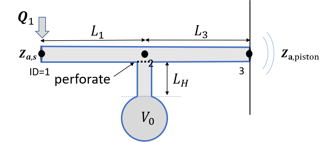
myPerf    = ac1D.PerforatedLayer(thickness,holeR,Ac,porosity = porosity)
myResPerf = ac1D.HelmholtzResonator(V0,LH,R,air,0.85,end_impedance=myPerf.radiation_impedance)

When we calculate and plot the radiation impedance

Za       = myResPerf.radiation_impedance(xdata.data)

we see that the resonance is around .

Radiation impedance of Helmholtz resonator in the T-joint example

The detailed tubes are defined as follows, including the reference tube:

tube1 = ac1D.AcousticTube(L1,air,A1)
tube3 = ac1D.AcousticTube(L3,air,A1)
end3  = acR.CircularPiston(R1,air)
entry4free  =  air.acoustic_FE(xdata,A1,ID=[1])

tube_ref = ac1D.AcousticTube(L1+L3,air,A1)

From those systems the elements are created with

elem1 = tube1.acoustic_FE(xdata,ID=[1,2])
elem3 = tube3.acoustic_FE(xdata,ID=[2,3])
rad3  =  end3.acoustic_FE(xdata,ID=[3])
entry4free  =  air.acoustic_FE(xdata,A1,ID=[1])

helmPerf = myResPerf.acoustic_FE(xdata,[2])

elem_ref = tube_ref.acoustic_FE(xdata,ID=[1,3])

Empty VAmodels and source are created as in the expansion chamber example. We solve both models and determine the insertion loss with

pow_out = tube_network.power(1,3,boundary = rad3) #free
pow_ref = tube_ref.power(1,3,boundary = rad3)

IL = pow_out.transfer(pow_ref,IDs=[3,3])
IL.plot(2,res='dB')

Leading to the following figure

Insertion loss of T-joint example