In contrast to pipe networks the chance for side paths is much lower in infinite layer systems.
A typical example application is the design of sound absorption systems.
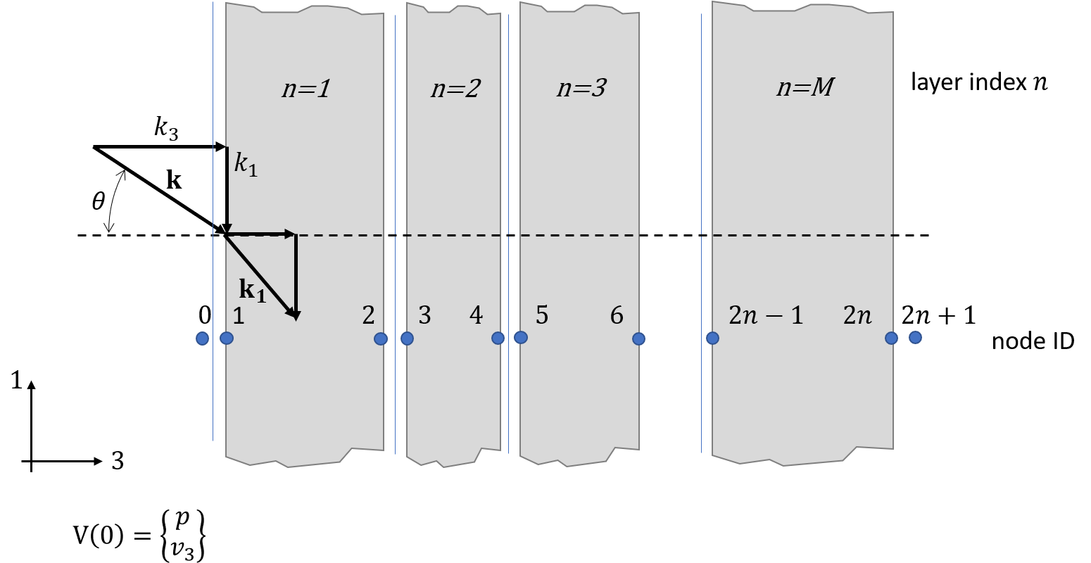
Infinite layers are a special version of one-dimensional system. Such system are one-dimensional in that
sense, that the properties change in one dimension and remain constant for the other two space dimensions.
The systems or layers are supposed to be infinite in those remaining two dimensions.
In contrast to acoustic networks from section Acoustic network there is an additional
variable required to describe the propagation parallel to the layers: the wavenumber perpendicular to the main dimension.
In the first version of pyva TMM was restricted to fluid layer, i.e. layers that can be described by fluid state variables
pressure and velocity. Note, that a this plate can also be described by fluid variable when no friction is considered.
The current version of pyva has implemented SolidLayer and
PoroElasticLayer. In addition, the Allard approach is implemented that
allows the combination of multiple layers of different nature. In the last examples of this section
the new possibilities will be shown.
The result can be plotted and shows the typical effects. The thick fibre layer provides excellent absorption
even at low frequencies. When we take the thinner version we loose low frequency performance.
In order to improve this we take the perforate cover, but here we loose the high frequency performance due to impedance mismatch at higher
frequencies.
However, the design of absorbers at given space and weight restrictions is an art. Pyva can support here and provide the tools for absorber design.
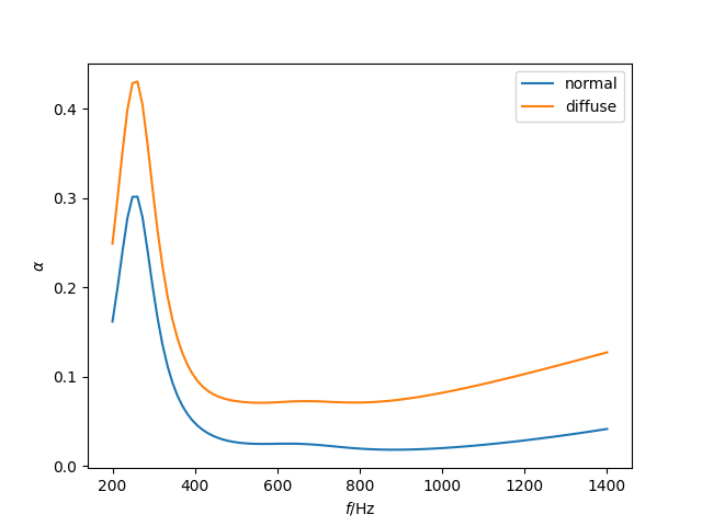
Diffuse absorption of different absorber configurations.
Double walls are the master tool set for efficient acoustic isolation.
Infinite layers are an excellent option to calculate the performance of double walls even though the
theory fails for example for single plates at the coincidence frequency. In such cases a full SEA model
in twin chamber configuration as in Two rooms separated by a wall section is recommended.
However, for fast and comparative studies on sound isolation the infinite layer in combination with the transfer matrices
is very useful.
# Fluid layerair_5cm=iL.FluidLayer(0.05,air)fibre_5cm=iL.FluidLayer(0.05,fibre1)# Limp mass layerheavy_1kg=iL.MassLayer(0.001,1000)heavy_2kg7=iL.MassLayer(0.001,2700)# Plate layeriL_alu1mm=iL.PlateLayer(alu1mm,)
All these layers are compiled in four different versions:
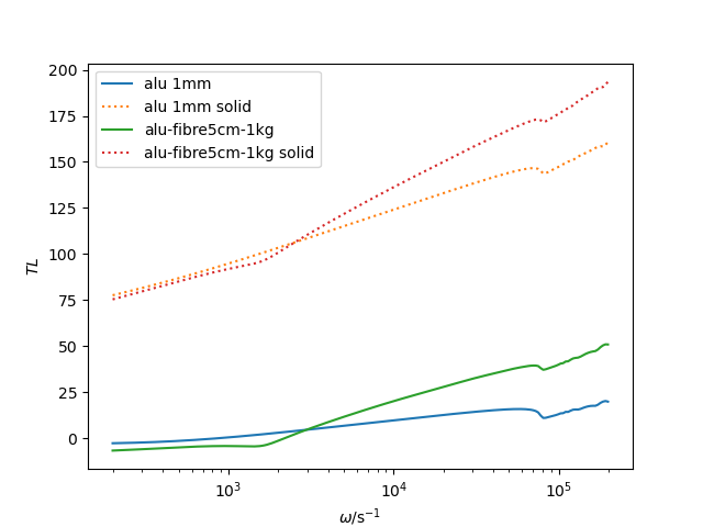
Plotting the results in the following figure shows the tremendous increase of isolation above the
double wall resonance. However, in addition is becomes obvious that the inner cavity requires damping and that
the lower resonance frequencies provide a much better performance in the mid-frequency.
Transmission loss of different single and double wall configurations.
The implementation of Brouards and Allards theory that allows layups of different nature.
Thus examples for such set-ups are required.
We used the carpet-impervious screen-fibre layup of [All2009] in section 11.7.2.
The layup is shown in the following figure.
# Create lay-up as TMmodelTMM_layup=mds.TMmodel((carpet1,carpet2,screen,fibre))
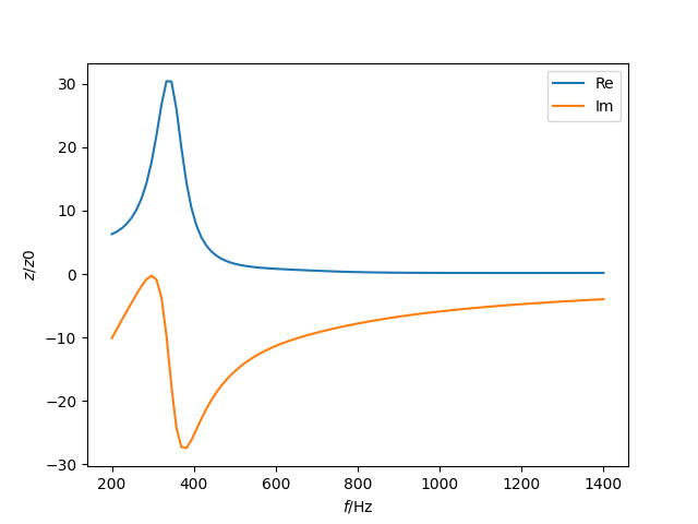
The impedance is calculated using the Allard version of the surface impedance calculation:
# Calculate normal surface impedanceZ=TMM_layup.impedance_allard(omega,kx=0,signal=False)
which gives the following result in accordance with [All2009] except the frequency unit.
Normal impedance of layup from [All2009] as in figure 11.17
With the following command the normal and diffuse absorption can be caluclated
# Calculate normal absorptionalpha0=TMM_layup.absorption(omega,kx=0.0,signal=False,allard=True)# Calculate diffure absorptionalpha_diff=TMM_layup.absorption_diffuse(omega,theta_max=np.pi*78/180,theta_step=np.pi/180,signal=False,allard=True)
Note the allard=True keyword argument required to use the Allard method of the absorption calculation.
The figure reveals that there are better absorbers in the world.
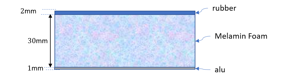
Acoustic transmission design with poroelastic foam and rubber
A practical version double wall systems is a so called mass-spring system.
Such layup consist of a soft foam covered by a heavy layer, e.g. rubber.
With the Allard theory poroelaxtic foams can be investigated in detail.
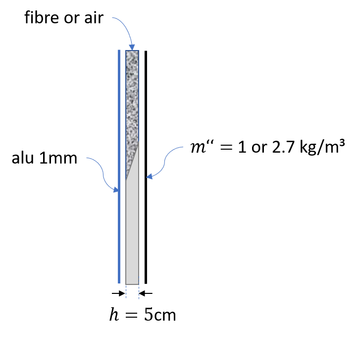
An example layup is shown in the following figure.
Every layer is given as plate, so that we can try different options:
# plate propertiesalu_1mm=stPC.PlateProp(0.001,alu)rubber_2mm=stPC.PlateProp(0.002,rubber)# test the foam as solidfoam_3cm_solid=stPC.PlateProp(0.03,melamin_vac)
We define the melamin foam either as PoroElasticLayer or SolidLayer
whereas the aluminium plate and the rubber layer are given as SolidLayer or ImperviousScreenLayer
# rubber and alu as solid- and screen layeriL_rubber_solid_2mm=iL.SolidLayer(rubber_2mm)iL_rubber_imper_2mm=iL.ImperviousScreenLayer(rubber_2mm)iL_alu_solid_1mm=iL.SolidLayer(alu_1mm)iL_alu_imper_1mm=iL.ImperviousScreenLayer(alu_1mm)
For the decoupling we create a super thin layer of low mass
# Mass of Fluid as gapiL_nothing=iL.MassLayer(1e-6,1.)
First we are interested in the impact of the solid or screen layer modelling
# TMmpodel using the solid or impervious screen formulationalu_melamin_rubber_solid=mds.TMmodel((iL_alu_solid_1mm,iL_foam_3cm,iL_rubber_solid_2mm))alu_melamin_rubber_imper=mds.TMmodel((iL_alu_imper_1mm,iL_foam_3cm,iL_rubber_imper_2mm))
and two other variations that decouple the alu plate of model the melamin foam as solid - neglecting the fluid waves.
Transmission loss of alu + mass-spring system using different modelling options
First, the difference between the versions modelling both skins as solid or screen is low.
Second, decoupling the alu from the foam leads to very different results. As a consequence this means that the
connection iof the noise control treatment must be exactly known to get correct results. This is also true for
experiments where the treatment must be carefully glued to the plate to get correct results.
Third, when the foam is modelled as solid the result is different, but the difference is lower than compared to the decoupling
effect.
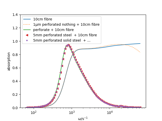
Calculating the diffuse field absorption coefficient and plotting the results gives the following figure:
Effect of plates that are perforated and allow bending dynamics
We see that due to the high mass of the steel plate the absorption is very similar except some small
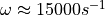
coincidence effects at .
The thin micron foil has nearly no impact as it moved with the flow and therefore there is no flow through the
perforation. There is only a minor impact at high frequencies.


 .
The thin micron foil has nearly no impact as it moved with the flow and therefore there is no flow through the
perforation. There is only a minor impact at high frequencies.
.
The thin micron foil has nearly no impact as it moved with the flow and therefore there is no flow through the
perforation. There is only a minor impact at high frequencies.